ARIMA model
ARIMA(\(p,d,q\)) extends ARMA(\(p,q\)) to non-stationary series by differencing \(d\) times. The \(d\) differences remove stochastic trends (unit roots), leaving a stationary series to which the ARMA(\(p,q\)) is applied. It is the most widely used model class for univariate time series forecasting.
Definition
A series \(y_t\) follows an ARIMA(\(p,d,q\)) if \(w_t = \Delta^d y_t = (1-L)^d y_t\) follows a stationary ARMA(\(p,q\)):
\[\Phi(L)(1-L)^d y_t = \Theta(L)\varepsilon_t\]
\[\Phi(L) = 1 - \phi_1 L - \cdots - \phi_p L^p, \qquad \Theta(L) = 1 + \theta_1 L + \cdots + \theta_q L^q\]
The three parameters:
- \(p\): AR order (number of autoregressive lags).
- \(d\): degree of differencing (integration order). \(d=0\) gives ARMA; \(d=1\) is the most common case.
- \(q\): MA order (number of moving average terms).
Special cases: ARIMA(1,0,0) = AR(1); ARIMA(0,1,0) = random walk; ARIMA(0,1,1) = exponentially weighted moving average (EWMA).
The Box-Jenkins methodology
The systematic procedure for identifying and fitting ARIMA models, proposed by Box and Jenkins (1970):
Step 1: Identification. Plot the series. Apply log or Box-Cox if variance is non-constant. Test for unit roots (ADF, KPSS). Difference \(d\) times until stationary. Examine ACF and PACF of the differenced series to identify candidate \(p\) and \(q\).
Step 2: Estimation. Fit the candidate ARIMA(\(p,d,q\)) by MLE. Compare models by AIC and BIC.
Step 3: Diagnostics. Check residuals are white noise: ACF of residuals, Ljung-Box test. If residuals show autocorrelation, revise \(p\) or \(q\).
Step 4: Forecasting. Use the fitted model to produce point forecasts and prediction intervals. Once real outcomes are observed, compare them against the forecast with standard regression evaluation metrics such as MAE, RMSE or MAPE.
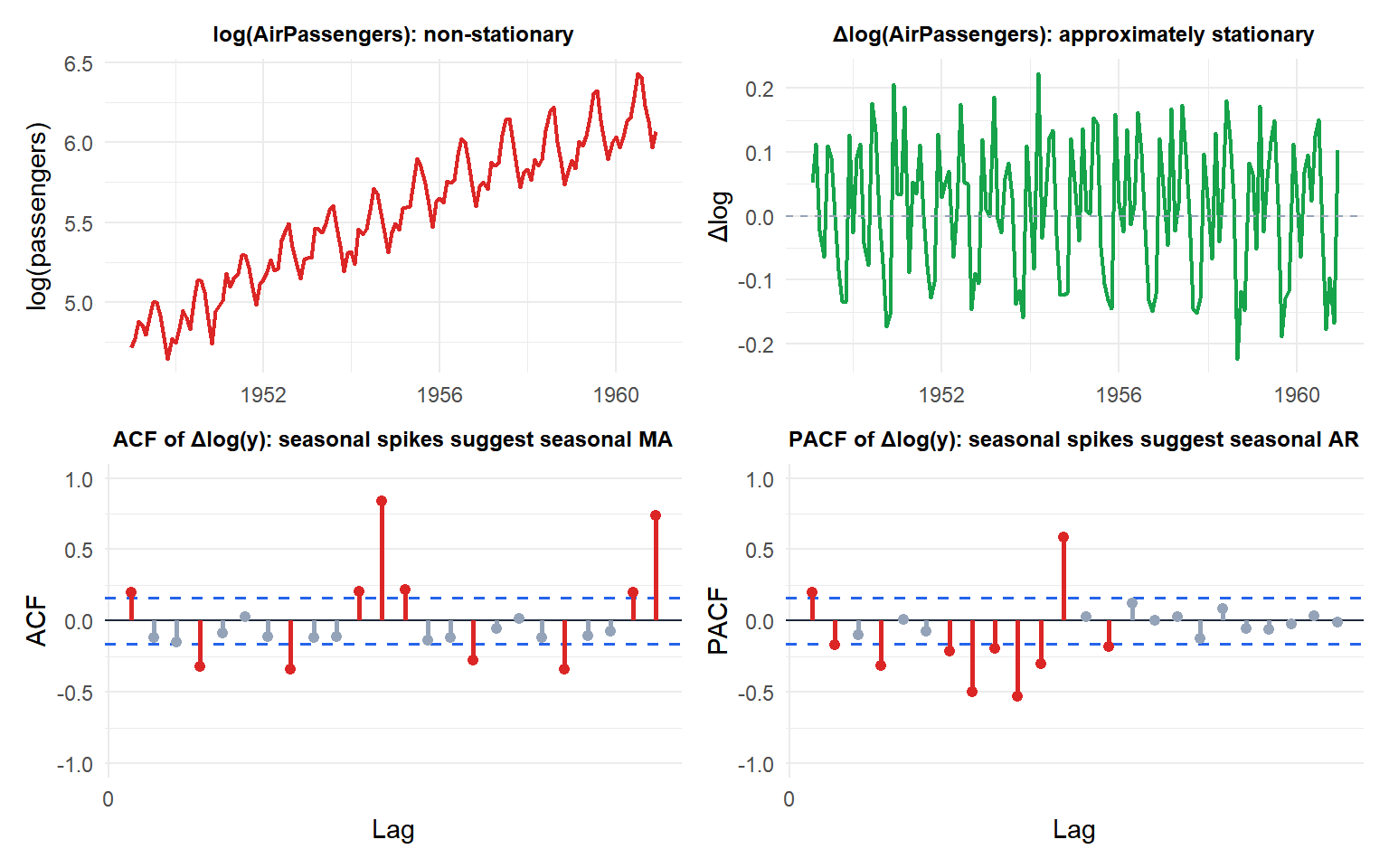
The original log series is non-stationary (upward trend). After one difference it is approximately stationary. The ACF and PACF of \(\Delta\log(y)\) still show seasonal spikes at lags 12, 24, suggesting a seasonal extension (SARIMA) is needed.
Choosing d
\(d\) is determined by unit root testing:
- Apply ADF and KPSS to the original series.
- If non-stationary, difference once and retest.
- Stop when both tests agree the series is stationary.
- For most economic and financial series, \(d = 1\) suffices. \(d = 2\) is rare and often indicates over-differencing.
In R: forecast::ndiffs(y) automates this using sequential ADF tests.
⚠️ Over-differencing makes forecasts worse
Applying \(d = 2\) when \(d = 1\) is sufficient introduces a unit root in the MA polynomial, producing unstable parameter estimates and forecasts that fan out excessively. Signs of over-differencing: the ACF of \(\Delta^d y_t\) starts at a large negative value at lag 1.
Under-differencing (using \(d = 0\) for a series that needs \(d = 1\)) produces non-stationary residuals with drifting mean and growing variance.
Example: ARIMA(1,1,1)
Fit an ARIMA(1,1,1) to the monthly US unemployment rate (a classic non-stationary economic series).
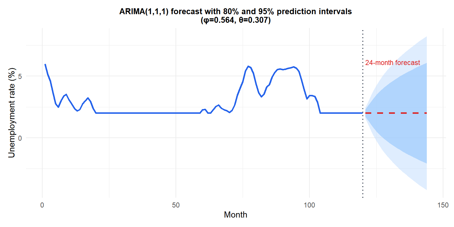
Prediction intervals widen with horizon: ARIMA(1,1,1) forecasts revert toward the recent trend, with uncertainty growing linearly in variance. The 80% (darker) and 95% (lighter) bands reflect this.
ARIMA vs ARMA
| ARMA(\(p,q\)) | ARIMA(\(p,d,q\)) | |
|---|---|---|
| Requires stationarity | Yes | No (handles \(I(d)\) series) |
| Handles trends | No | Yes (via differencing) |
| Long-run forecast | Reverts to constant mean | Follows a stochastic trend |
| \(d = 0\) special case | Yes (ARIMA = ARMA) | - |
💡 ARIMA in R
# Manual specification
arima(y, order = c(1, 1, 1))

# Automatic selection by AIC (Box-Jenkins automated)
library(forecast)
auto.arima(y)

# Diagnose residuals
checkresiduals(fit)

# Forecast 12 periods ahead
forecast(fit, h = 12)
auto.arima() applies the Box-Jenkins methodology automatically: it tests for unit roots to choose \(d\), then searches over \((p, q)\) by AIC. It is the recommended starting point for any ARIMA analysis.