Ljung-Box test
The Ljung-Box test checks whether the residuals of a fitted time series model are white noise: uncorrelated across all lags. A significant result means the model has not captured all the autocorrelation structure in the data and needs refinement.
Context: when is this test used?
After fitting a time series model (ARIMA, exponential smoothing, regression with time series errors), the residuals should be uncorrelated. If they are not, the model is misspecified: it is leaving predictable structure in the errors, which means forecasts and standard errors are unreliable.
The Ljung-Box test formalizes this diagnostic check. It is not used to test whether raw data are autocorrelated (use the ACF for that), but to test whether the residuals of a fitted model are.
Test statistic
\[Q = n(n+2) \sum_{k=1}^{m} \frac{\hat{r}_k^2}{n-k}\]
where \(n\) is the number of observations, \(m\) is the number of lags tested, and \(\hat{r}_k\) is the sample autocorrelation at lag \(k\). Under \(H_0\) (no autocorrelation), \(Q \sim \chi^2(m - p - q)\), where \(p\) and \(q\) are the AR and MA orders of the fitted model (both 0 if testing raw data).
The Ljung-Box statistic is a weighted sum of squared autocorrelations, giving more weight to lags with fewer observations (\(n-k\) in the denominator). This makes it more sensitive than the original Box-Pierce statistic, which uses \(n\sum \hat{r}_k^2\) without the correction.
Hypotheses: \(H_0\): the residuals are independently distributed (no autocorrelation at any lag up to \(m\)). \(H_1\): at least one autocorrelation \(\hat{r}_k\) is non-zero.
The ACF plot: the visual companion
The Ljung-Box test gives a single p-value for all lags up to \(m\). The ACF plot shows the individual autocorrelations at each lag, making it easy to see where the structure is. Always use both together.
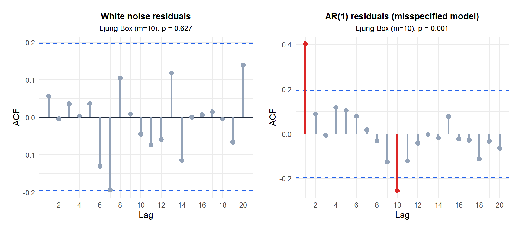
Red bars exceed the 95% confidence bands (dashed blue lines). White noise residuals have no significant bars and a large p-value. Autocorrelated residuals show a clear pattern decaying from lag 1, with a very small p-value.
Complete example: ARIMA model diagnostics
Monthly airline passenger numbers (Box-Jenkins dataset, \(n = 144\)) are fitted with an ARIMA(1,1,1)(1,1,1)[12] model. The Ljung-Box test is applied to the residuals.
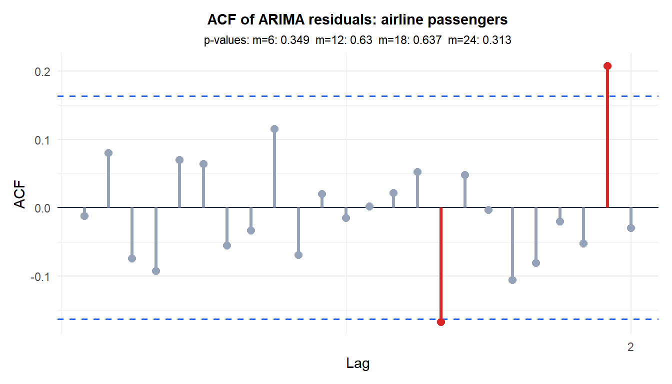
All p-values are well above 0.05: the residuals show no significant autocorrelation. The model has adequately captured the data’s structure.
Choosing the number of lags \(m\)
⚠️ The choice of m matters and there is no single correct answer
Testing too few lags misses autocorrelations at higher lags. Testing too many reduces power because the chi-squared distribution has more degrees of freedom, making it harder to detect any single significant autocorrelation.
Common rules of thumb:
- For non-seasonal series: \(m = \min(10, n/5)\).
- For seasonal series with period \(s\): \(m = 2s\) (e.g., \(m = 24\) for monthly data).
- For ARIMA\((p,d,q)\) models: use \(df = m - p - q\) degrees of freedom in the chi-squared distribution.
In R, Box.test(..., fitdf = p + q) applies the degrees of freedom correction automatically.
Running the test in R
# After fitting an ARIMA model
fit <- arima(x, order = c(1, 1, 1))
resid <- residuals(fit)

# Ljung-Box test with degrees of freedom correction
Box.test(resid, lag = 10, type = "Ljung-Box", fitdf = 2)  # fitdf = p + q

# Multiple lags at once
sapply(c(6, 12, 18, 24), function(m)
  Box.test(resid, lag = m, type = "Ljung-Box", fitdf = 2)$p.value)

# ACF plot for visual inspection
acf(resid, lag.max = 24)
💡 Interpreting the result in context
A significant Ljung-Box result (\(p \leq 0.05\)) means the model has residual autocorrelation. Typical next steps:
- Inspect the ACF and PACF of the residuals to identify which lags are significant.
- Increase the AR or MA order of the model.
- For seasonal patterns, add seasonal AR or MA terms.
- If all else fails, consider a different model class (e.g., GARCH for financial returns with volatility clustering).
A non-significant result does not guarantee the model is correct: it only says the residuals are consistent with white noise up to lag \(m\).

