Regression evaluation metrics (MAE, MSE, RMSE, MAPE, WAPE)

Classification models get judged by a confusion matrix and ROC/AUC. Regression and forecasting models, where the prediction is a number rather than a class, are judged by how far off that number tends to be. MAE, MSE, RMSE, MAPE and WAPE are the five metrics that answer that, and they do not always agree on which model is better.

MAE, MSE and RMSE

These three all work directly with the prediction errors \(e_i = y_i - \hat{y}_i\), in the original units of \(y\), or in squared units for MSE:

MAE treats every unit of error the same. MSE squares the error first, so a single large miss contributes far more than several small ones, which makes MSE (and RMSE, its square root, back in the original units of \(y\)) much more sensitive to outliers than MAE. RMSE is the most commonly reported of the three because it is in the same units as \(y\) while still penalizing large errors heavily, a useful middle ground.

MAPE and WAPE: percentage-based metrics

MAE, MSE and RMSE are all scale-dependent: an RMSE of 50 is excellent for predicting house prices and catastrophic for predicting daily coffee sales. MAPE and WAPE fix this by expressing error as a percentage of the actual value, which makes them comparable across series or datasets on completely different scales:

The difference looks small, MAPE averages the individual percentage errors, WAPE sums the absolute errors and the absolute actuals separately before dividing, but it has a large practical consequence covered below.

Worked example: a biased, noisy forecast

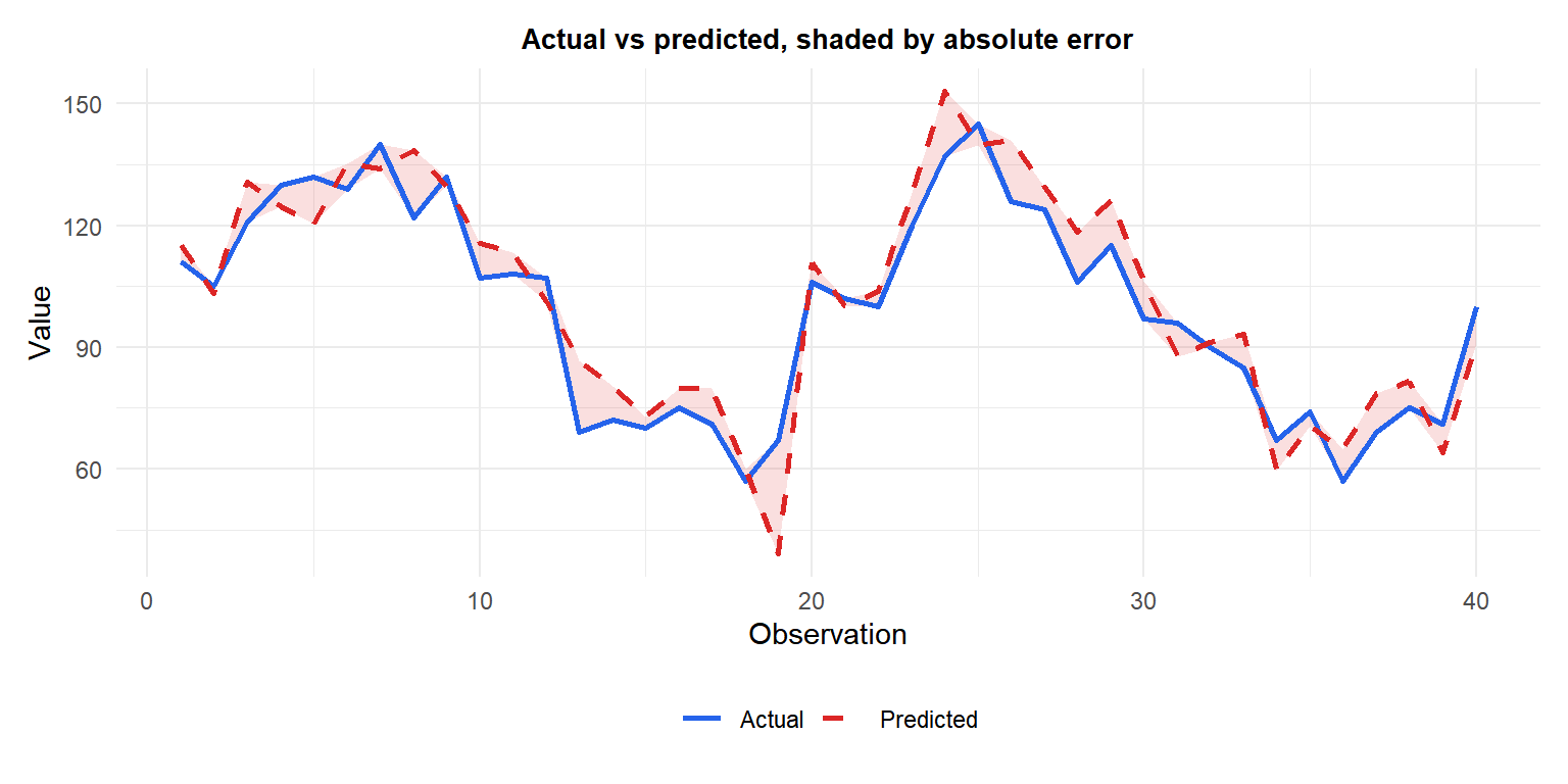
Computing all five metrics on the exact same predictions shows how they rank the same errors differently.

Computing all five metrics on the same forecast

A simulated series of \(n=40\) actual values (ranging from 57 to 145) and a forecast with a small upward bias (average forecast about 2 units too high) plus random noise. All five metrics computed on the same data:

Metric	Value
MAE	7.95
MSE	89.64
RMSE	9.47
MAPE	8.64%
WAPE	7.97%

Here MAPE and WAPE roughly agree, both say the typical error is around 8% of the actual value, because every actual value in this series is comfortably far from zero (minimum 57).

Where MAPE breaks and WAPE does not

MAPE divides by each individual actual value, so a forecast target that is sometimes close to zero makes MAPE explode, even if the absolute error at that point is tiny.

This is why WAPE (also called weighted MAPE) is the standard choice in demand forecasting and retail, where individual products or days with near-zero actual sales are routine, not an edge case. MAPE remains useful when every actual value is safely away from zero and a percentage is still more interpretable than raw units.

Running it in R

None of these have a single universal base R function, they are each a one-line formula:

mae  <- mean(abs(actual - pred))
mse  <- mean((actual - pred)^2)
rmse <- sqrt(mse)
mape <- mean(abs((actual - pred) / actual)) * 100
wape <- sum(abs(actual - pred)) / sum(abs(actual)) * 100

# Packages that bundle all of them, with consistent naming
library(Metrics)
mae(actual, pred); rmse(actual, pred)

library(yardstick)
# yardstick works on a data frame of truth/estimate columns