ROC curve and AUC
A classifier produces a score for each observation. Converting scores to class labels requires choosing a threshold. The ROC curve shows how sensitivity and specificity trade off as the threshold varies across its entire range. AUC summarizes this curve in a single number: the probability that the model ranks a random positive case higher than a random negative case.
From scores to predictions: the confusion matrix
A binary classifier assigns each observation a score \(\hat{p} \in [0,1]\) and predicts positive if \(\hat{p} \geq t\) for some threshold \(t\). The resulting predictions are summarized in the confusion matrix:
| Predicted positive | Predicted negative | |
|---|---|---|
| Actually positive | TP | FN |
| Actually negative | FP | TN |
Key metrics derived from the confusion matrix:
\[\text{Sensitivity (Recall, TPR)} = \frac{TP}{TP+FN} \quad \text{(of all positives, how many did we catch?)}\]
\[\text{Specificity} = \frac{TN}{TN+FP}, \quad \text{FPR} = 1 - \text{Specificity} = \frac{FP}{FP+TN}\]
\[\text{Precision (PPV)} = \frac{TP}{TP+FP} \quad \text{(of all predicted positives, how many are truly positive?)}\]
\[\text{Accuracy} = \frac{TP+TN}{n}\]
The threshold \(t\) controls the tradeoff: lower \(t\) catches more positives (high TPR) but also misclassifies more negatives (high FPR).
The ROC curve
The Receiver Operating Characteristic (ROC) curve plots TPR (sensitivity) on the y-axis against FPR (1-specificity) on the x-axis, for every possible threshold \(t \in [0,1]\).
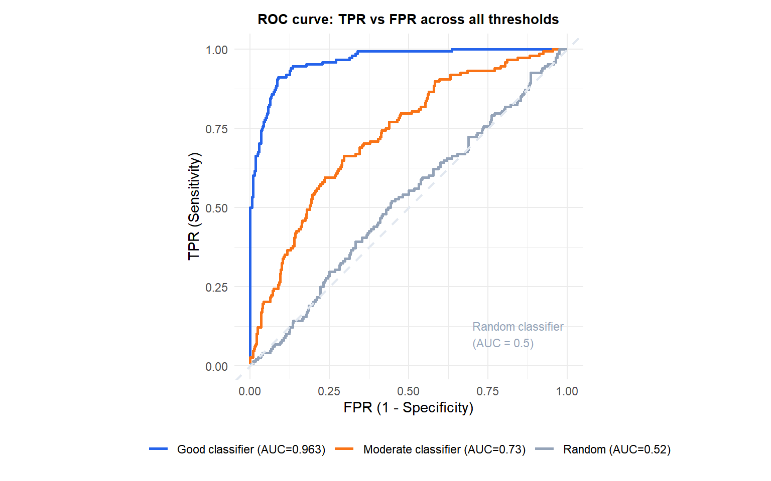
The diagonal line represents a random classifier (AUC = 0.5): it achieves the same TPR as FPR at every threshold, gaining nothing from the scores. A perfect classifier would reach the top-left corner (TPR=1, FPR=0) and have AUC=1. The further the curve bulges toward the top-left, the better the classifier.
AUC: area under the ROC curve
The AUC (Area Under the Curve) is the integral of the ROC curve:
\[\text{AUC} = \int_0^1 \text{TPR}(\text{FPR}^{-1}(t))\, dt\]
It has a clean probabilistic interpretation (Wilcoxon-Mann-Whitney statistic):
\[\text{AUC} = P(\hat{p}_+ > \hat{p}_-)\]
The probability that a randomly chosen positive case receives a higher score than a randomly chosen negative case. AUC = 0.5: random ranking. AUC = 1: perfect ranking. AUC = 0: perfectly reversed ranking.
This interpretation makes AUC threshold-independent: it measures the quality of the score ranking, not the quality of any specific threshold decision.
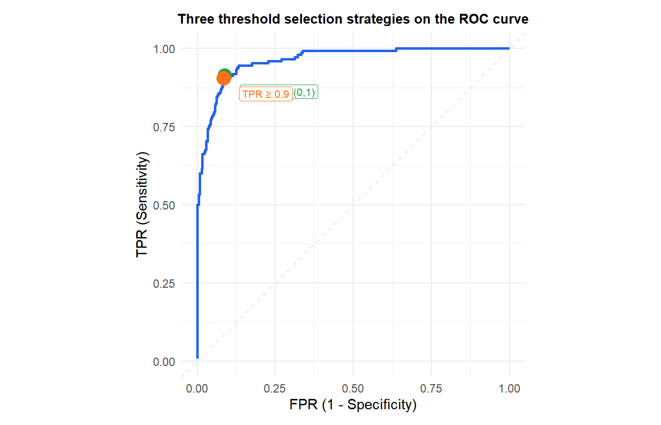
Choosing an operating threshold
AUC evaluates overall ranking quality but real decisions require a threshold. How to choose \(t\):
- Equal cost: maximize accuracy, or equivalently find the threshold closest to the top-left corner of the ROC curve (minimum distance to \((0,1)\)).
- Cost-sensitive: if a false negative is \(c\) times more costly than a false positive, the optimal threshold satisfies the slope condition on the ROC curve.
- Youden’s J index: maximize \(J = \text{TPR} - \text{FPR} = \text{Sensitivity} + \text{Specificity} - 1\).
- Domain constraint: fix a maximum acceptable FPR (e.g., in screening, accept at most 10% false positives) and find the threshold that maximizes TPR under that constraint.
Precision-Recall curve
For highly imbalanced datasets (e.g., fraud detection where 0.1% of cases are positive), ROC and AUC can be misleading: a classifier that labels everything as negative achieves FPR=0 and a high AUC while being completely useless.
The Precision-Recall (PR) curve plots precision vs recall across thresholds. It focuses on the positive class and is more informative when:
- The dataset is highly imbalanced.
- The cost of false negatives and false positives are very different.
- The rare class is the class of interest.
The average precision (AP) summarizes the PR curve, analogous to AUC for the ROC curve.
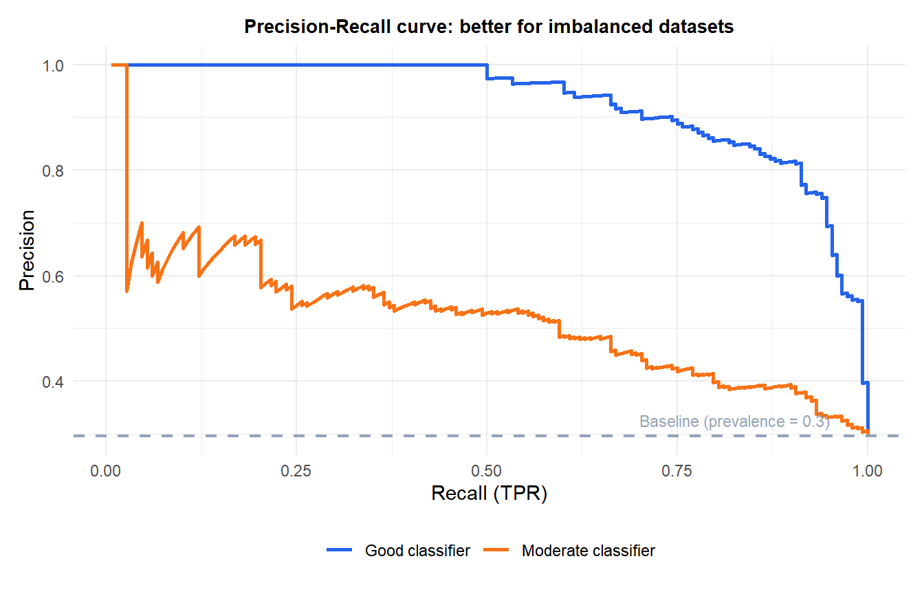
The baseline (dashed) is the precision achieved by randomly predicting positive with probability equal to the prevalence. A useful classifier must stay well above this line.
⚠️ AUC is not the right metric when classes are severely imbalanced
Consider a fraud detection system where 0.1% of transactions are fraudulent. A classifier that always predicts “not fraud” achieves accuracy = 99.9%, AUC close to 0.5 (slightly above, because random guessing respects the imbalance). But average precision could be near zero.
Use precision-recall AUC (or average precision) instead of ROC-AUC when:
- The positive class is rare (prevalence \(< 5\)-10%).
- You care primarily about detecting the rare class.
- False positives have very different costs from false negatives.
Also: when comparing models with AUC, check whether the difference is statistically significant. The DeLong test compares two ROC curves and provides a p-value for the difference in AUC.
💡 ROC and AUC in R
library(pROC)

# ROC curve and AUC
roc_obj <- roc(y_true, scores, levels=c(0,1), direction="<")
auc(roc_obj)                         # AUC value
ci.auc(roc_obj)                      # 95% CI for AUC
plot(roc_obj, col="#2563EB")         # ROC plot

# Compare two ROC curves
roc1 <- roc(y_true, scores1)
roc2 <- roc(y_true, scores2)
roc.test(roc1, roc2)                 # DeLong test

# Optimal threshold by Youden's J
coords(roc_obj, "best", best.method="youden")

# Precision-Recall
library(PRROC)
pr_obj <- pr.curve(scores.class1=scores[y_true==1],
                   scores.class0=scores[y_true==0],
                   curve=TRUE)
pr_obj$auc.integral   # average precision
plot(pr_obj)

# Full evaluation with caret
library(caret)
confusionMatrix(pred_labels, true_labels, positive="1")
