Probability density function
The probability density function (PDF) describes how probability is distributed across the possible values of a continuous random variable. The PDF itself is not a probability, but its integral over any interval gives the probability of the variable falling in that interval.
Definition
A function \(f(x)\) is the probability density function of a continuous random variable \(X\) if:
\[ P(a \leq X \leq b) = \int_{a}^{b} f(x)\, dx \quad \text{for any } a \leq b \]
In plain terms: the probability that \(X\) falls between \(a\) and \(b\) is the area under the curve of \(f(x)\) from \(a\) to \(b\).
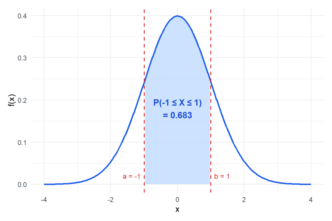
Figure 1: Probability as area under the curve: P(−1 ≤ X ≤ 1) ≈ 0.683 for a standard normal distribution
⚠️ f(x) is not a probability, it can be greater than 1
This is the most frequent misunderstanding about PDFs. The value (f(x)) is a density, not a probability. Probabilities come from integrating, not from evaluating (f(x)) directly.
As a consequence, there is no upper bound on \(f(x)\): a uniform distribution on \([0, 0.1]\) has \(f(x) = 10\) everywhere on that interval, and that is perfectly valid. The integral still equals 1:
\[\int_0^{0.1} 10\, dx = 10 \times 0.1 = 1\]
The only constraint is \(f(x) \geq 0\) and \(\int_{-\infty}^{\infty} f(x)\, dx = 1\).
Properties of the PDF
A function \(f(x)\) is a valid PDF if and only if:
- \(f(x) \geq 0\) for all \(x\).
- \(\int_{-\infty}^{\infty} f(x)\, dx = 1\).
From the definition, additional properties follow:
- \(P(X = x) = 0\) for any single point (the integral over a single point is zero).
- \(P(a \leq X \leq b) = P(a < X \leq b) = P(a \leq X < b) = P(a < X < b)\): strict vs non-strict inequalities are equivalent for continuous variables.
💡 How to check if a function is a valid PDF
Common PDFs
Normal distribution
The most important distribution in statistics. Its PDF is:
\[f(x) = \frac{1}{\sigma\sqrt{2\pi}} e^{-\frac{(x-\mu)^2}{2\sigma^2}}\]
The bell-shaped curve is symmetric around \(\mu\). There is no closed-form expression for its integral, so probabilities are computed numerically or from tables.
Exponential distribution
Models waiting times and lifetimes of systems with constant failure rate:
\[f(x) = \lambda e^{-\lambda x} \quad \text{for } x \geq 0\]
The parameter \(\lambda > 0\) is the rate. The mean is \(1/\lambda\).
Uniform distribution
All values in \([a, b]\) are equally likely:
\[f(x) = \frac{1}{b-a} \quad \text{for } a \leq x \leq b\]
The simplest continuous distribution. Its integral from \(a\) to \(b\) gives \((b-a) \cdot \frac{1}{b-a} = 1\).
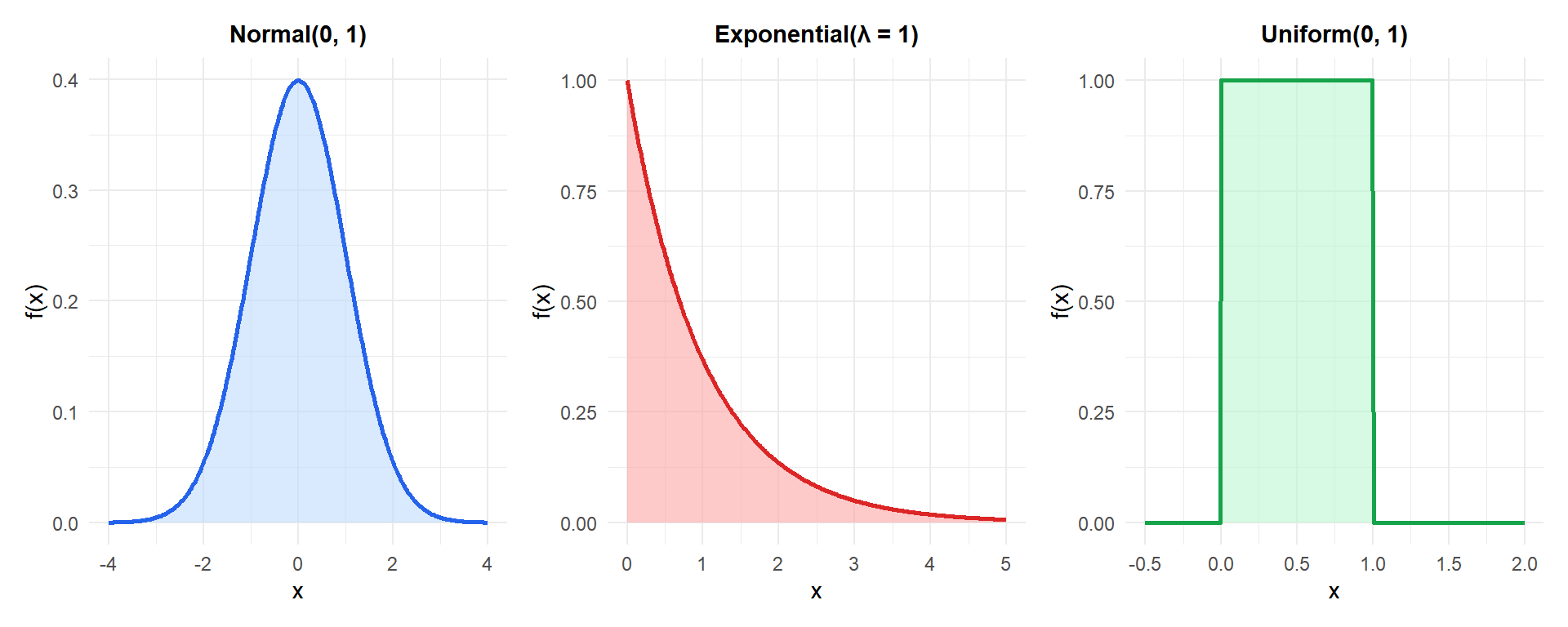
Figure 2: Three common probability density functions: normal (left), exponential (center), and uniform (right)
Calculating probabilities from the PDF
Example 1: uniform distribution
A bus arrives at a stop uniformly distributed between 0 and 10 minutes from now. What is the probability of waiting between 2 and 6 minutes?
The PDF is \(f(x) = 1/10\) for \(0 \leq x \leq 10\).
\[P(2 \leq X \leq 6) = \int_2^6 \frac{1}{10}\, dx = \frac{1}{10} \times (6-2) = 0.4\]
There is a 40% chance of waiting between 2 and 6 minutes.
Example 2: exponential distribution
A customer service call lasts an exponentially distributed time with mean 5 minutes (\(\lambda = 0.2\)). What is the probability the call lasts less than 3 minutes?
\[P(X \leq 3) = \int_0^3 0.2\, e^{-0.2x}\, dx = \left[-e^{-0.2x}\right]_0^3 = 1 - e^{-0.6} \approx 0.451\]
About 45% of calls end within the first 3 minutes.
Is (f(x) = 2x) for (0 \leq x \leq 1) (and zero elsewhere) a valid PDF?
Check non-negativity: \(2x \geq 0\) for \(x \in [0,1]\). ✓
Check normalization: \[\int_0^1 2x\, dx = \left[x^2\right]_0^1 = 1 - 0 = 1 \checkmark\]
Yes, it is a valid PDF. It assigns more probability to values near 1 than near 0.
What is \(P(0.5 \leq X \leq 1)\)?
\[P(0.5 \leq X \leq 1) = \int_{0.5}^1 2x\, dx = \left[x^2\right]_{0.5}^1 = 1 - 0.25 = 0.75\]
Relationship with the CDF
The PDF and the CDF are two sides of the same coin:
\[F(x) = \int_{-\infty}^x f(t)\, dt \qquad \text{and} \qquad f(x) = \frac{d}{dx}F(x)\]
The CDF is the integral of the PDF; the PDF is the derivative of the CDF. Given one, you can always find the other (as long as \(F\) is differentiable).

