Complementary events

The complement of an event \(A\) is the event that \(A\) does not occur. It always has probability \(1 - P(A)\), and it is often the easiest way to solve problems involving “at least one” or “at least once” scenarios.

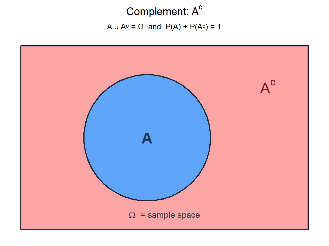
Definition

Let \(A\) be an event on a sample space \(\Omega\). The complement of \(A\), written \(A^c\) or \(\bar{A}\), is the event containing all outcomes in \(\Omega\) that are not in \(A\):

Its probability follows directly from the fact that \(A\) and \(A^c\) partition the sample space:

Three properties always hold:

• \(A \cup A^c = \Omega\) (exhaustive: one of them must occur).
• \(A \cap A^c = \emptyset\) (mutually exclusive: they cannot both occur).
• \(P(A) + P(A^c) = 1\).

The complement trick

The complement is most useful when calculating \(P(A)\) directly requires summing many cases, but \(P(A^c)\) reduces to a single calculation. The standard pattern:

\[P(A) = 1 - P(A^c)\]

This works whenever \(A\) involves “at least one”, “at least once”, or “more than zero” occurrences, because the complement is “none” or “zero”, which is usually a single term.

At least one defective item

A shipment contains 50 items, 8 of which are defective. Five items are sampled without replacement. What is the probability that at least one is defective?

Direct calculation requires summing \(P(X=1) + P(X=2) + \cdots + P(X=5)\), five hypergeometric terms.

Using the complement: \(A^c\) = no defectives in the sample.

\[P(A^c) = \frac{\binom{42}{5}}{\binom{50}{5}} = \frac{850668}{2118760} \approx 0.401\]

\[P(\text{at least one defective}) = 1 - 0.401 = 0.599\]

One calculation instead of five.

At least one server failure in a month

A server has a 0.5% daily failure probability, independent across days. What is the probability of at least one failure in 30 days?

Direct: sum 30 binomial terms. Using the complement:

\[P(\text{no failures in 30 days}) = (1 - 0.005)^{30} = 0.995^{30} \approx 0.860\]

\[P(\text{at least one failure}) = 1 - 0.860 = 0.140\]

About 14% chance of at least one outage in a month.

More examples

Quality control: batch acceptance

A quality standard requires rejecting a batch if it contains any item outside tolerance. A machine produces items out of tolerance with probability 0.03, independently. A batch of 20 items is tested.

\(P(\text{batch rejected}) = P(\text{at least one out of tolerance})\)

\[= 1 - P(\text{all within tolerance}) = 1 - (0.97)^{20} \approx 1 - 0.544 = 0.456\]

About 46% of batches are rejected. If the defect rate is improved to 1%:

\[1 - (0.99)^{20} \approx 1 - 0.818 = 0.182\]

The rejection rate drops to 18%. Small improvements in the defect rate have a large effect on batch acceptance.

Password security: brute force attack

A system locks an account after 5 failed login attempts. An attacker tries random passwords. Each attempt succeeds with probability \(p = 0.001\).

\(P(\text{account not compromised in 5 attempts}) = P(\text{all 5 fail})\)

\[= (1 - 0.001)^5 = 0.999^5 \approx 0.995\]

\[P(\text{compromised}) = 1 - 0.995 = 0.005\]

Only 0.5% chance per attack session. But if 10,000 accounts are attacked:

\[P(\text{at least one compromised}) = 1 - 0.995^{10000} \approx 1 - e^{-50} \approx 1\]

At scale, breaches are near-certain. This is why rate limiting alone is not enough.

Clinical trial: at least one adverse event

In a trial with 200 patients, each has a 2% probability of experiencing an adverse event, independently.

\[P(\text{at least one adverse event}) = 1 - (0.98)^{200} \approx 1 - 0.0176 = 0.982\]

There is a 98% probability that at least one patient in the trial experiences an adverse event, even though each individual risk is low. This is why rare side effects are still expected to appear in trials of any reasonable size.