Lagrange multipliers
Lagrange multipliers convert a constrained optimization problem into an unconstrained system of equations. The key geometric insight: at the constrained optimum, the objective function and the constraint share the same tangent, meaning their gradients are parallel. The multiplier measures how much the optimal value changes when the constraint is relaxed.
Geometric intuition
Consider minimizing \(f(x,y)\) subject to \(g(x,y) = 0\). The constraint defines a curve in \(\mathbb{R}^2\). As we move along this curve, \(f\) changes. The constrained minimum occurs where we can no longer decrease \(f\) by moving along the constraint.
At any point on the constraint, we can decompose motion into two components: along the constraint (tangential) and perpendicular to it (normal). The gradient \(\nabla g\) is perpendicular to the constraint curve. At the constrained optimum, the tangential component of \(\nabla f\) must be zero: otherwise we could move along the constraint to decrease \(f\). This means \(\nabla f\) has no component along the constraint, i.e., \(\nabla f\) is perpendicular to the constraint too. Since both \(\nabla f\) and \(\nabla g\) are perpendicular to the constraint, they must be parallel:
\[\nabla f(x^*) = \lambda \nabla g(x^*)\]
for some scalar \(\lambda\) (the Lagrange multiplier).
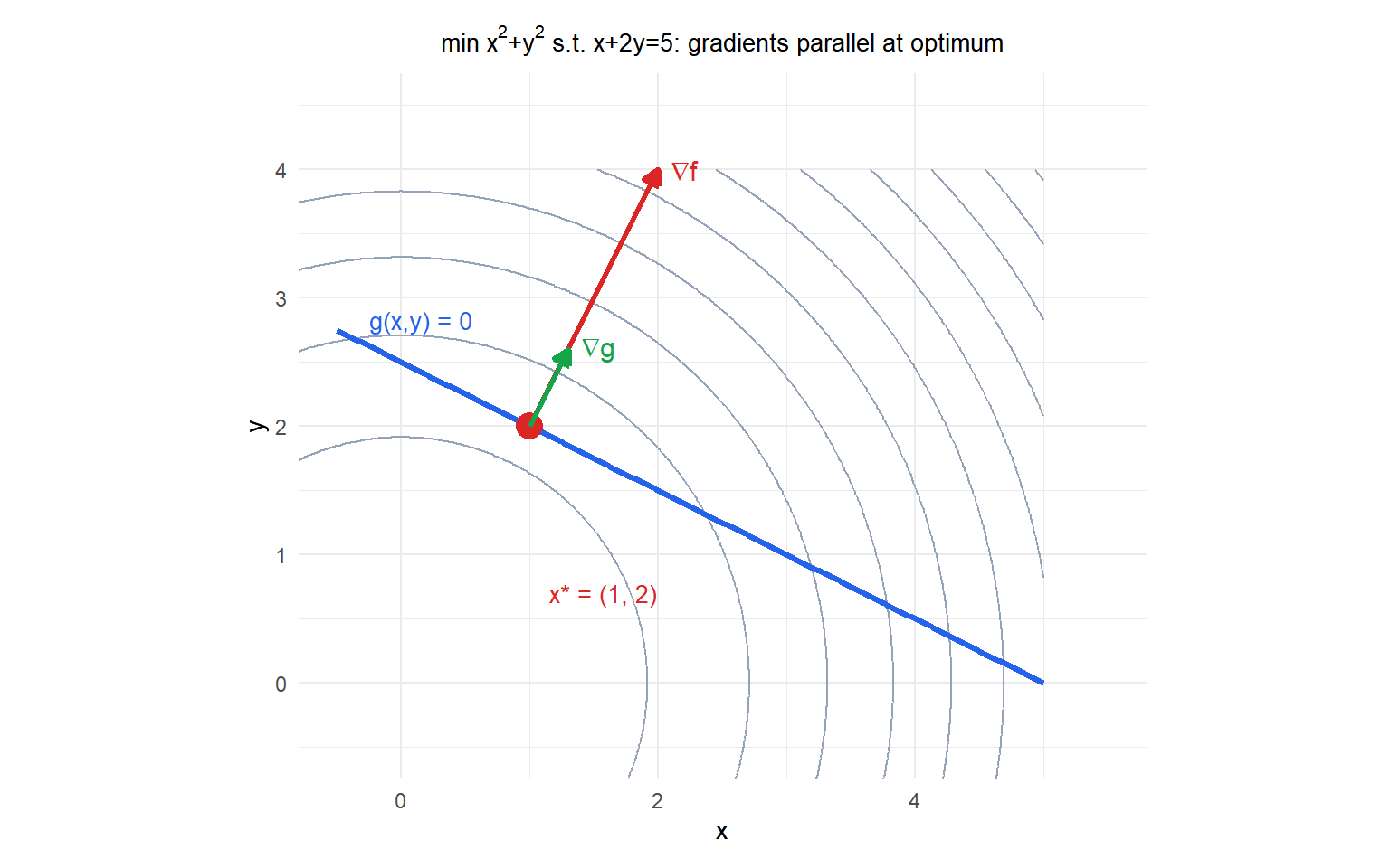
At the optimum \((1,2)\), \(\nabla f = (2, 4)\) and \(\nabla g = (1, 2)\) are parallel: \(\nabla f = 2\nabla g\), so \(\lambda^* = 2\). The level curves of \(f\) (circles) are tangent to the constraint line at the optimal point.
The Lagrangian
The method of Lagrange multipliers introduces the Lagrangian function:
\[\mathcal{L}(x, \lambda) = f(x) + \lambda g(x)\]
The constrained optimum is a stationary point of \(\mathcal{L}\) with respect to both \(x\) and \(\lambda\). Setting all partial derivatives to zero gives the Lagrange conditions:
\[\frac{\partial \mathcal{L}}{\partial x_i} = \frac{\partial f}{\partial x_i} + \lambda \frac{\partial g}{\partial x_i} = 0 \quad \forall i\]
\[\frac{\partial \mathcal{L}}{\partial \lambda} = g(x) = 0\]
The second condition simply enforces the constraint. Together these give \(n+1\) equations in \(n+1\) unknowns \((x_1, \ldots, x_n, \lambda)\).
Example 1: minimum distance to a line
Minimize \(f(x,y) = x^2 + y^2\) (squared distance from the origin) subject to \(g(x,y) = x + 2y - 5 = 0\).
Lagrangian: \(\mathcal{L} = x^2 + y^2 + \lambda(x + 2y - 5)\).
First-order conditions:
\[\frac{\partial \mathcal{L}}{\partial x} = 2x + \lambda = 0 \implies x = -\lambda/2\]
\[\frac{\partial \mathcal{L}}{\partial y} = 2y + 2\lambda = 0 \implies y = -\lambda\]
\[\frac{\partial \mathcal{L}}{\partial \lambda} = x + 2y - 5 = 0\]
Substituting \(x = -\lambda/2\) and \(y = -\lambda\) into the constraint:
\[-\lambda/2 + 2(-\lambda) = 5 \implies -5\lambda/2 = 5 \implies \lambda = -2\]
Therefore \(x^* = 1\), \(y^* = 2\), \(f^* = 1^2 + 2^2 = 5\).
The closest point on the line \(x + 2y = 5\) to the origin is \((1, 2)\), at distance \(\sqrt{5}\).
Multiple equality constraints
With \(m\) equality constraints \(g_j(x) = 0\), \(j=1,\ldots,m\), the Lagrangian becomes:
\[\mathcal{L}(x, \lambda) = f(x) + \sum_{j=1}^m \lambda_j g_j(x)\]
\[\nabla_x \mathcal{L} = \nabla f(x) + \sum_{j=1}^m \lambda_j \nabla g_j(x) = 0\]
\[g_j(x) = 0, \quad j = 1, \ldots, m\]
This gives \(n + m\) equations in \(n + m\) unknowns. The geometric interpretation extends: at the optimum, \(\nabla f\) lies in the subspace spanned by \(\{\nabla g_1, \ldots, \nabla g_m\}\).
Example 2: utility maximization (budget constraint)
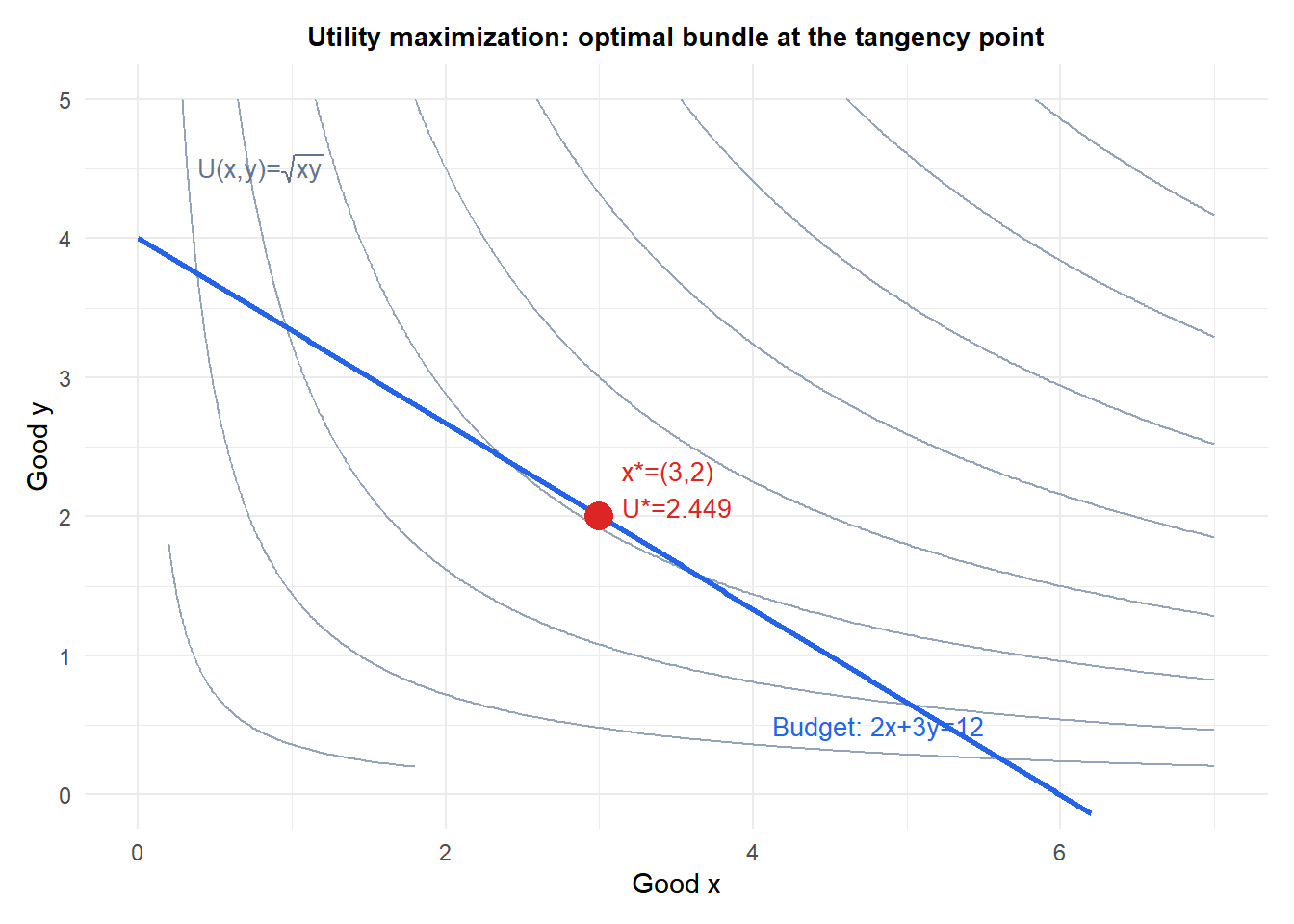
A consumer maximizes utility \(U(x,y) = x^{0.5} y^{0.5}\) (Cobb-Douglas) subject to a budget constraint \(2x + 3y = 12\) (prices 2 and 3, income 12).
Lagrangian: \(\mathcal{L} = x^{0.5}y^{0.5} + \lambda(12 - 2x - 3y)\).
First-order conditions:
\[\frac{\partial \mathcal{L}}{\partial x} = \frac{1}{2}x^{-0.5}y^{0.5} - 2\lambda = 0 \implies \frac{y^{0.5}}{2x^{0.5}} = 2\lambda\]
\[\frac{\partial \mathcal{L}}{\partial y} = \frac{1}{2}x^{0.5}y^{-0.5} - 3\lambda = 0 \implies \frac{x^{0.5}}{2y^{0.5}} = 3\lambda\]
Dividing the first by the second: \(\frac{y}{x} = \frac{2}{3} \cdot \frac{2}{1} = \frac{4}{3}\)… Actually dividing gives \(y/x = (2\lambda \cdot 2)/(2\lambda \cdot 3) \cdot (x^{0.5}/y^{0.5})\). Let us use the MRS condition directly:
\[\frac{MU_x}{MU_y} = \frac{p_x}{p_y} \implies \frac{y}{x} = \frac{2}{3} \implies y = \frac{2x}{3}\]
Substituting into the budget constraint: \(2x + 3 \cdot \frac{2x}{3} = 12 \implies 4x = 12 \implies x^* = 3\), \(y^* = 2\).
Optimal utility: \(U^* = \sqrt{3 \cdot 2} = \sqrt{6} \approx 2.449\). Multiplier: \(\lambda^* = \frac{y^{0.5}}{4x^{0.5}} = \frac{\sqrt{2}}{4\sqrt{3}} = \frac{1}{4}\sqrt{2/3} \approx 0.204\).
Economic interpretation of the multiplier
The Lagrange multiplier \(\lambda^*\) measures the sensitivity of the optimal value to the constraint:
\[\lambda^* = \frac{df^*}{db}\]
where \(b\) is the RHS of the constraint \(g(x) = b\). If the constraint is \(g(x) = 0\) and we relax it to \(g(x) = \varepsilon\), the optimal value changes by approximately \(\lambda^* \varepsilon\).
In the utility example: \(\lambda^* \approx 0.204\) means that increasing the budget by €1 increases optimal utility by approximately 0.204 units. This is exactly the concept of shadow price in linear programming: the dual variables are Lagrange multipliers of the LP constraints.
This interpretation makes multipliers economically meaningful: they are the marginal value of relaxing each constraint by one unit.
Constraint qualification
The Lagrange conditions are necessary for optimality, but they require a regularity condition called constraint qualification (CQ). The most common is the Linear Independence CQ (LICQ): the gradients \(\nabla g_1(x^*), \ldots, \nabla g_m(x^*)\) must be linearly independent at the optimal point.
If LICQ fails (e.g., two constraints are tangent to each other at the optimum), the Lagrange multipliers may not exist or may not be unique. In such cases, the method fails to find the correct optimum.
⚠️ Lagrange conditions are necessary but not sufficient in general
For non-convex problems, a point satisfying the Lagrange conditions could be a local minimum, local maximum, or saddle point. Always verify the second-order conditions or check that the problem is convex.
For convex problems (convex \(f\), affine constraints), any point satisfying the Lagrange conditions is a global minimum. This is the most important practical case: when \(f\) is convex and the constraints are linear, the Lagrange conditions give the global optimum.
Extension to inequality constraints: KKT
Lagrange multipliers handle only equality constraints. For inequality constraints \(g_i(x) \leq 0\), the extension is the Karush-Kuhn-Tucker (KKT) conditions, which add:
- Dual feasibility: \(\lambda_i \geq 0\) for inequality constraints.
- Complementary slackness: \(\lambda_i g_i(x^*) = 0\) for each \(i\). Either the constraint is active (\(g_i = 0\), any \(\lambda_i \geq 0\)) or the multiplier is zero (\(\lambda_i = 0\), constraint inactive).
KKT unifies Lagrange multipliers (equality constraints, any \(\lambda\)) with the inequality case (\(\lambda \geq 0\), complementary slackness). It is the fundamental optimality condition for constrained optimization.
💡 Lagrange multipliers in R
library(nloptr)

# Minimize f(x,y) = x^2 + y^2 subject to x + 2y = 5
f    <- function(x) x[1]^2 + x[2]^2
grad_f <- function(x) c(2*x[1], 2*x[2])
h    <- function(x) x[1] + 2*x[2] - 5   # equality constraint = 0

res <- nloptr(x0 = c(0, 0),
              eval_f = f,
              eval_grad_f = grad_f,
              eval_g_eq = h,
              opts = list(algorithm="NLOPT_LD_SLSQP", xtol_rel=1e-8))
res$solution   # c(1, 2)
res$objective  # 5

# For linear constraints: use lpSolve or CVXR
# For general nonlinear: use nloptr with SLSQP or COBYLA
