Dynamic programming
Dynamic programming (DP) solves optimization problems by breaking them into overlapping subproblems, solving each subproblem once, and storing the result. It converts exponential-time recursive algorithms into polynomial-time ones. The key insight: if the overall optimal solution can be built from optimal solutions to subproblems, DP applies.
Two conditions for dynamic programming
DP works when a problem has two properties:
1. Optimal substructure
The optimal solution to the problem contains optimal solutions to its subproblems. This is Bellman’s principle of optimality: an optimal policy has the property that whatever the initial state and decision are, the remaining decisions must constitute an optimal policy with regard to the state resulting from the first decision.
If you can construct the optimal solution to the whole problem from optimal solutions to smaller instances, the problem has optimal substructure.
2. Overlapping subproblems
The recursive solution solves the same subproblems repeatedly. This is what distinguishes DP from divide and conquer (which also uses optimal substructure but has non-overlapping subproblems, e.g., merge sort).
If the same subproblems appear many times, storing their solutions (memoization or tabulation) avoids redundant computation and reduces exponential time to polynomial.
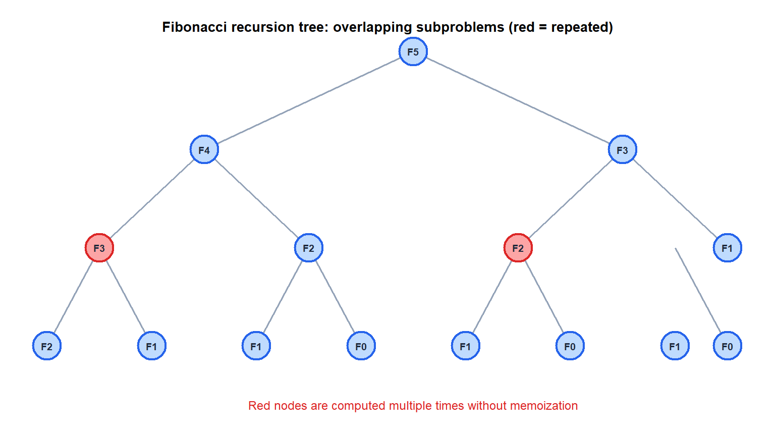
Without memoization, computing \(F_n\) takes \(O(2^n)\) time. With memoization, each of the \(n\) distinct subproblems is solved once: \(O(n)\) time.
Top-down vs bottom-up
There are two equivalent ways to implement DP:
Top-down (memoization)
Write the recursive solution naturally. Add a cache (hash table or array) to store results of subproblems as they are computed. Before solving a subproblem, check if its result is already cached.
memo <- c()
fib <- function(n) {
  if (n <= 1) return(n)
  if (!is.na(memo[n])) return(memo[n])
  result <- fib(n-1) + fib(n-2)
  memo[n] <<- result
  result
}
Advantage: only computes subproblems that are actually needed. Disadvantage: recursive call stack overhead; can hit stack limits for large \(n\).
Bottom-up (tabulation)
Fill a table of subproblem solutions in order from smallest to largest. Each entry is computed using previously filled entries.
fib_dp <- function(n) {
  if (n <= 1) return(n)
  dp <- numeric(n+1)
  dp[1] <- 0; dp[2] <- 1
  for (i in 3:(n+1)) dp[i] <- dp[i-1] + dp[i-2]
  dp[n+1]
}
Advantage: no recursion overhead; naturally iterative; easier to analyze space complexity. Disadvantage: computes all subproblems even if some are not needed.
In practice, bottom-up is usually preferred for its simplicity and efficiency.
Example 1: 0/1 knapsack
\(n\) items with values \(v_i\) and weights \(w_i\). Knapsack capacity \(W\). Maximize total value subject to weight limit. Each item is either taken (1) or not (0).
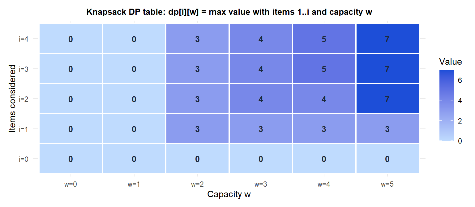
Substructure: define \(dp[i][w]\) = maximum value using items \(1,\ldots,i\) with capacity \(w\).
Recurrence:
\[dp[i][w] = \begin{cases} dp[i-1][w] & \text{if } w_i > w \text{ (item } i \text{ does not fit)} \\ \max(dp[i-1][w],\; v_i + dp[i-1][w-w_i]) & \text{otherwise} \end{cases}\]
Base case: \(dp[0][w] = 0\) for all \(w\) (no items, no value).
Time complexity: \(O(nW)\) (pseudopolynomial: polynomial in \(n\) and \(W\), but exponential in the number of bits of \(W\)).
| Item | Value | Weight |
|---|---|---|
| 1 | 3 | 2 |
| 2 | 4 | 3 |
| 3 | 5 | 4 |
| 4 | 6 | 5 |
DP table \(dp[i][w]\):
| w=0 | w=1 | w=2 | w=3 | w=4 | w=5 | |
|---|---|---|---|---|---|---|
| i=0 | 0 | 0 | 0 | 0 | 0 | 0 |
| i=1 | 0 | 0 | 3 | 3 | 3 | 3 |
| i=2 | 0 | 0 | 3 | 4 | 4 | 7 |
| i=3 | 0 | 0 | 3 | 4 | 5 | 7 |
| i=4 | 0 | 0 | 3 | 4 | 5 | 7 |
Optimal value: \(dp[4][5] = 7\) (take items 1 and 2: \(3+4=7\), \(2+3=5 \leq W\)).
Example 2: Longest Common Subsequence (LCS)
Given two strings \(X = x_1\ldots x_m\) and \(Y = y_1\ldots y_n\), find the longest subsequence common to both (not necessarily contiguous).
Substructure: define \(dp[i][j]\) = length of LCS of \(X[1..i]\) and \(Y[1..j]\).
Recurrence:
\[dp[i][j] = \begin{cases} 0 & i=0 \text{ or } j=0 \\ dp[i-1][j-1] + 1 & x_i = y_j \\ \max(dp[i-1][j],\; dp[i][j-1]) & x_i \neq y_j \end{cases}\]
Time and space: \(O(mn)\) for both. The LCS itself is recovered by backtracking through the table.
LCS length = 4 (e.g., BCAB or BDAB). The DP table fills in \(O(7 \times 5) = 35\) cells instead of checking all \(2^7 = 128\) subsequences of \(X\).
Connection with Dijkstra
Dijkstra’s algorithm is a special case of dynamic programming. The shortest path from \(s\) to \(v\) satisfies:
\[d[v] = \min_{u: (u,v) \in E} \{d[u] + w(u,v)\}\]
This is a DP recurrence: the shortest path to \(v\) is built from the shortest path to its predecessor \(u\). The optimal substructure property holds because any subpath of a shortest path is itself a shortest path.
The difference from generic DP: Dijkstra exploits the non-negativity of weights to process subproblems in order of increasing distance, avoiding the need to fill a full \(|V| \times |V|\) table.
More generally, shortest paths on DAGs (directed acyclic graphs) can be solved with a simple DP in topological order: \(O(V+E)\), faster than Dijkstra’s \(O((V+E)\log V)\).
When DP does not apply
⚠️ DP requires optimal substructure: not all problems have it
The classic counterexample: longest simple path in a general graph. Unlike shortest paths, longest paths do not have optimal substructure. Knowing the longest path from \(s\) to an intermediate vertex \(u\) does not help find the longest path from \(s\) to \(v\) through \(u\): combining two long paths may create a cycle (visiting a vertex twice), violating the simple path requirement.
Longest simple path is NP-hard in general graphs, while shortest path is solvable in polynomial time precisely because of optimal substructure.
Before applying DP, verify that the optimal solution to the whole problem truly depends only on optimal solutions to subproblems, with no interference between subproblem solutions.
Complexity and the curse of dimensionality
DP trades time for space: it stores solutions to all subproblems. The state space determines both time and space complexity. For a DP with \(k\) state variables each taking \(O(n)\) values, the table has \(O(n^k)\) entries: exponential in the number of state variables.
This is the curse of dimensionality in DP: adding one state variable multiplies the table size by \(n\). For continuous state spaces (stochastic control, reinforcement learning), the table is infinite and approximations are required.
Practical strategies to manage state space: rolling arrays (keep only the last row of the DP table), space-time tradeoffs, state compression for bitmask DP.
💡 Dynamic programming in R
# 0/1 Knapsack
knapsack_dp <- function(values, weights, W) {
  n  <- length(values)
  dp <- matrix(0, nrow=n+1, ncol=W+1)
  for (i in 1:n) {
    for (w in 1:W) {
      dp[i+1, w+1] <- dp[i, w+1]
      if (weights[i] <= w)
        dp[i+1, w+1] <- max(dp[i+1, w+1],
                            values[i] + dp[i, w-weights[i]+1])
    }
  }
  list(value=dp[n+1, W+1], table=dp)
}

knapsack_dp(c(3,4,5,6), c(2,3,4,5), W=5)$value  # 7

# LCS length
lcs_length <- function(X, Y) {
  m <- nchar(X); n <- nchar(Y)
  X <- strsplit(X,"")[[1]]; Y <- strsplit(Y,"")[[1]]
  dp <- matrix(0, m+1, n+1)
  for (i in 1:m) for (j in 1:n)
    dp[i+1,j+1] <- if(X[i]==Y[j]) dp[i,j]+1 else max(dp[i,j+1],dp[i+1,j])
  dp[m+1,n+1]
}

lcs_length("ABCBDAB", "BDCAB")  # 4
