Splines
Splines fit smooth curves to data by joining piecewise polynomials at locations called knots. They overcome the global rigidity of polynomial regression while avoiding the roughness of piecewise linear fits. Splines are the building blocks of GAMs and are used everywhere: from dose-response curves to growth models to flexible regression.
Why not just use a high-degree polynomial?
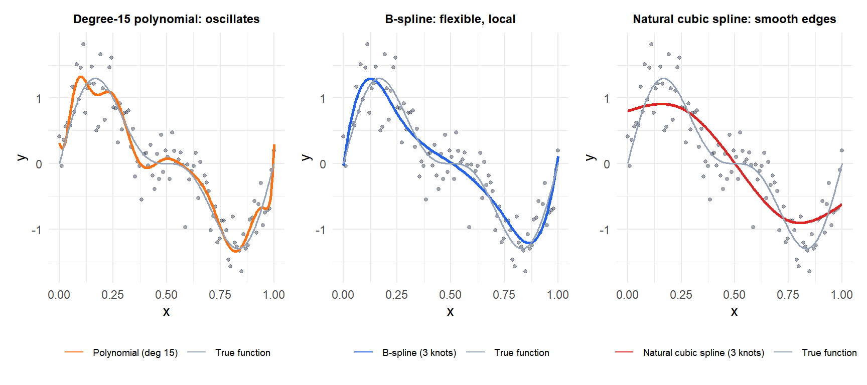
A global polynomial of degree \(d\) fitted to \(n\) points has only one set of coefficients for the entire range of \(x\). High-degree polynomials oscillate wildly at the boundaries (Runge’s phenomenon) and are sensitive to any single observation. Splines solve this by fitting low-degree (usually cubic) polynomials on subintervals, joined smoothly at knots.
The result: local flexibility without global instability.
Regression splines
A regression spline with \(K\) knots \(\xi_1 < \xi_2 < \cdots < \xi_K\) fits a separate polynomial on each interval \((-\infty, \xi_1)\), \([\xi_1, \xi_2)\), …, \([\xi_K, +\infty)\), with continuity constraints at each knot.
A cubic spline requires continuity of the function and its first and second derivatives at each knot. This gives \(K+4\) free parameters (4 for the base cubic, \(K\) additional jump terms). The basis representation uses truncated power functions:
\[h(x, \xi) = (x - \xi)_+^3 = \begin{cases}(x-\xi)^3 & x > \xi \\ 0 & x \leq \xi\end{cases}\]
The spline is: \[f(x) = \beta_0 + \beta_1 x + \beta_2 x^2 + \beta_3 x^3 + \sum_{k=1}^K \gamma_k h(x, \xi_k)\]
This is a linear model in the basis functions: OLS applies directly.
Natural cubic spline: adds the constraint that the function is linear beyond the boundary knots (\(f'' = 0\) for \(x < \xi_1\) and \(x > \xi_K\)). This reduces boundary variance at the cost of a small bias, and is generally recommended over the unconstrained cubic spline.
Smoothing splines
Instead of choosing a fixed set of knots, a smoothing spline places a knot at every observed \(x_i\) and penalizes roughness:
\[\min_{f} \sum_{i=1}^n (y_i - f(x_i))^2 + \lambda \int [f''(x)]^2 dx\]
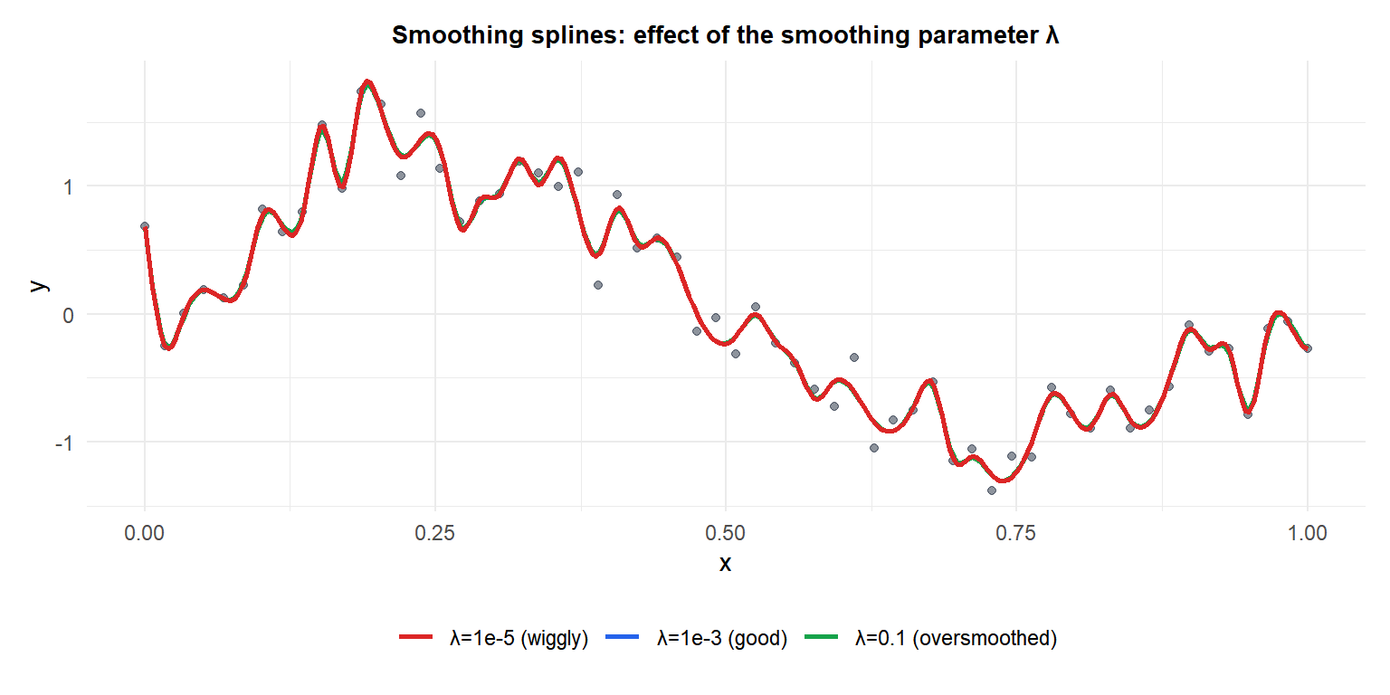
The penalty \(\lambda \int [f'']^2 dx\) discourages a wiggly \(f\). The solution is always a natural cubic spline with knots at each \(x_i\), regardless of \(\lambda\).
- \(\lambda = 0\): interpolates every point (maximum roughness, df = \(n\)).
- \(\lambda \to \infty\): approaches a straight line (minimum roughness, df = 2).
- Optimal \(\lambda\): chosen by leave-one-out cross-validation or generalized cross-validation (GCV), which minimizes prediction error on held-out points.
The effective degrees of freedom \(\text{df}_\lambda\) decreases from \(n\) to 2 as \(\lambda\) increases, providing an interpretable complexity measure.
Knot placement for regression splines
The number and location of knots is the key modelling decision:
- Fixed knots at quantiles: place \(K\) knots at evenly spaced quantiles of \(x\). Concentrates knots where data is dense. The most common default.
- Cross-validation: fit the model for several values of \(K\) and choose the one that minimizes CV error.
- Adaptive knot selection: methods like MARS (Multivariate Adaptive Regression Splines) search for the best knot locations automatically.
As a rule of thumb for regression splines: 3-5 knots at quantiles is usually sufficient for most applications. More knots do not always help and increase the risk of overfitting.
⚠️ Extrapolation beyond the boundary knots is unreliable
Regression splines behave well within the range of the data but extrapolate poorly outside the boundary knots, where the model has no constraint. Natural cubic splines are linear beyond the boundaries, which is a reasonable default. Standard cubic splines can curve sharply outside the data range.
Never use a spline for out-of-sample predictions beyond the observed range of \(x\) without careful inspection of the boundary behavior.
Connection with GAMs
A Generalized Additive Model (GAM) extends logistic and linear regression by replacing each linear term \(\beta_j x_j\) with a smooth function \(f_j(x_j)\):
\[g(E[y]) = \beta_0 + f_1(x_1) + f_2(x_2) + \cdots + f_k(x_k)\]
Each \(f_j\) is typically a smoothing spline or regression spline. Splines are the building blocks that make GAMs flexible: without them, GAMs reduce to standard GLMs.
💡 Splines in R
library(splines)

# Regression spline with bs() - B-spline basis
fit_bs <- lm(y ~ bs(x, knots=c(0.25, 0.5, 0.75), degree=3))

# Natural cubic spline with ns()
fit_ns <- lm(y ~ ns(x, df=5))        # df controls knot number
fit_ns <- lm(y ~ ns(x, knots=c(0.33, 0.67)))  # explicit knots

# Smoothing spline
fit_ss <- smooth.spline(x, y, cv=TRUE)  # cv=TRUE selects lambda by LOO-CV
plot(fit_ss)

# GAM with penalized splines (mgcv)
library(mgcv)
fit_gam <- gam(y ~ s(x1) + s(x2), data=df)
plot(fit_gam)  # shows each smooth component
