Nonlinear regression
Nonlinear regression fits models where at least one parameter appears nonlinearly in the prediction function. Unlike polynomial regression (which is linear in its parameters and solved by OLS), nonlinear models require iterative algorithms. The payoff is the ability to fit scientifically meaningful functional forms: growth curves, dose-response relationships, enzyme kinetics.
Linear in parameters vs linear in variables
The critical distinction is not whether the curve is straight, but whether the model is linear in the parameters:
- \(y = \beta_0 + \beta_1 x + \beta_2 x^2\): polynomial, but linear in \(\beta\). OLS applies directly.
- \(y = \beta_0 e^{\beta_1 x}\): exponential, nonlinear in \(\beta_1\). OLS does not apply; iterative methods required.
- \(y = \beta_0 + \beta_1 \log x\): log-transformed predictor, but linear in \(\beta\). OLS applies.
A model is linear if the gradient \(\partial f / \partial \beta_j\) does not depend on any \(\beta\). If it does, the model is nonlinear and requires nls() or similar.
The general nonlinear model:
\[y_i = f(x_i, \boldsymbol{\beta}) + \varepsilon_i, \qquad \varepsilon_i \sim N(0, \sigma^2)\]
where \(f\) is any smooth function, not necessarily linear in \(\boldsymbol{\beta}\). The parameters \(\hat{\boldsymbol{\beta}}\) minimize the residual sum of squares \(\sum_i (y_i - f(x_i, \boldsymbol{\beta}))^2\), but there is no closed-form solution.
Fitting algorithms
Gauss-Newton algorithm
Linearizes \(f\) around the current estimate \(\boldsymbol{\beta}^{(t)}\) using a first-order Taylor expansion:
\[f(x_i, \boldsymbol{\beta}) \approx f(x_i, \boldsymbol{\beta}^{(t)}) + \mathbf{J}_i^T (\boldsymbol{\beta} - \boldsymbol{\beta}^{(t)})\]
where \(\mathbf{J}_i = \partial f / \partial \boldsymbol{\beta}|_{\boldsymbol{\beta}^{(t)}}\) is the Jacobian. The update is:
\[\boldsymbol{\beta}^{(t+1)} = \boldsymbol{\beta}^{(t)} + (\mathbf{J}^T\mathbf{J})^{-1}\mathbf{J}^T \mathbf{r}^{(t)}\]
where \(\mathbf{r}^{(t)} = \mathbf{y} - f(\mathbf{x}, \boldsymbol{\beta}^{(t)})\) is the residual vector. Converges quadratically near the solution but can diverge if the initial values are far from the optimum.
Levenberg-Marquardt algorithm
A robust extension of Gauss-Newton that interpolates between Gauss-Newton (\(\lambda=0\)) and gradient descent (\(\lambda\) large):
\[\boldsymbol{\beta}^{(t+1)} = \boldsymbol{\beta}^{(t)} + (\mathbf{J}^T\mathbf{J} + \lambda \mathbf{I})^{-1}\mathbf{J}^T \mathbf{r}^{(t)}\]
The damping parameter \(\lambda\) is adjusted automatically: increased when a step fails (making it more like gradient descent, stable but slow) and decreased when a step succeeds (more like Gauss-Newton, fast near solution). This makes it much more robust to poor initial values. It is the default algorithm in nls().
Common nonlinear models
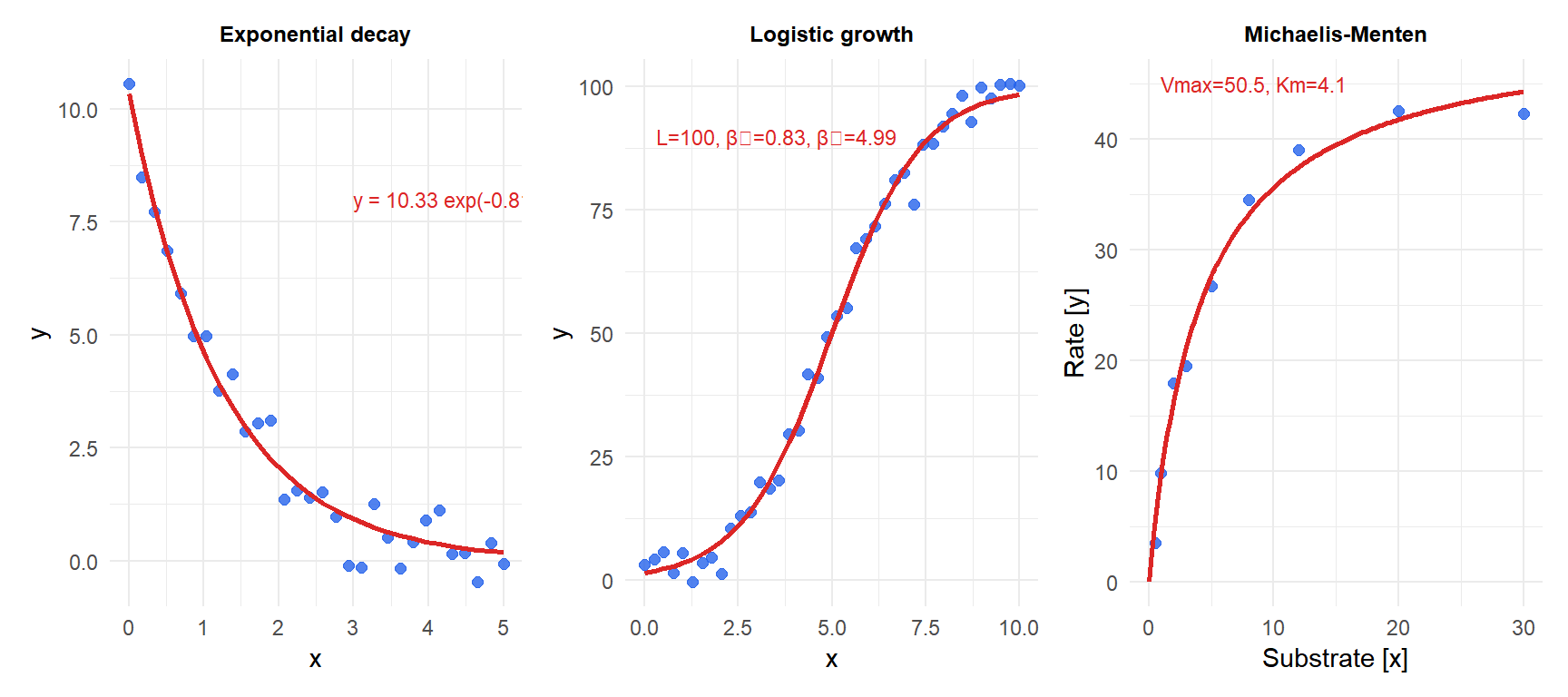
1. Exponential model
\[y = \beta_0 e^{\beta_1 x}\]
\(\beta_0 > 0\): initial value (\(y\) when \(x=0\)). \(\beta_1 > 0\): exponential growth; \(\beta_1 < 0\): exponential decay. Applications: radioactive decay, population growth, compound interest.
Linearization: \(\log y = \log \beta_0 + \beta_1 x\) is linear, so OLS on the log-transformed response is often used as a quick approximation. However, this minimizes the log-scale residuals, not the original scale residuals, and gives different (biased) estimates when \(\varepsilon\) is additive on the original scale.
2. Logistic growth model
\[y = \frac{L}{1 + e^{-\beta_1(x - \beta_2)}}\]
\(L\): carrying capacity (upper asymptote). \(\beta_1\): growth rate. \(\beta_2\): inflection point (\(x\) at which \(y = L/2\)). S-shaped curve. Applications: population growth, technology adoption, epidemic spread, dose-response.
3. Michaelis-Menten model
\[y = \frac{V_\text{max} \cdot x}{K_m + x}\]
\(V_\text{max}\): maximum rate (upper asymptote as \(x \to \infty\)). \(K_m\): half-saturation constant (\(x\) at which \(y = V_\text{max}/2\)). Applications: enzyme kinetics, nutrient uptake, pharmacokinetics.
Choosing initial values
Nonlinear regression can fail or converge to a local minimum if the initial parameter values are far from the true solution. Strategies for choosing good starting values:
- Use domain knowledge: for the logistic model, \(L\) is the observable upper asymptote; \(\beta_2\) is roughly where the curve is steepest.
- Linearize and use OLS: log-transform the exponential model and use the OLS slope and intercept as starting values.
- Grid search: evaluate the objective function on a grid of starting values and use the best as the starting point.
- Use self-starting models: R provides
SSlogis,SSasymp,SSmicmenetc., which estimate their own starting values automatically.
⚠️ Convergence failure usually means bad starting values or a wrong model
When nls() throws “singular gradient” or “step factor reduced below minimum”, the usual causes are:
- Initial values far from the optimum.
- The model is not identifiable from the data (parameters are confounded).
- The functional form is wrong for the data.
Always plot the data first and overlay the model with your starting values before fitting. If the starting curve looks reasonable, the algorithm has a good chance of converging. If it looks completely wrong, no algorithm will recover.
💡 Nonlinear regression in R
# Manual starting values
fit <- nls(y ~ b0 * exp(b1 * x), data=df,
           start=list(b0=10, b1=-0.5))
summary(fit)
confint(fit)

# Self-starting models (no starting values needed)
fit_logis <- nls(y ~ SSlogis(x, Asym, xmid, scal), data=df)
fit_mm    <- nls(y ~ SSmicmen(x, Vm, K), data=df)
fit_exp   <- nls(y ~ SSasymp(x, Asym, R0, lrc), data=df)

# Predictions and residual plot
plot(fitted(fit), residuals(fit))
abline(h=0, lty=2)

# More robust fitting with minpack.lm (Levenberg-Marquardt)
library(minpack.lm)
fit_lm <- nlsLM(y ~ b0*exp(b1*x), data=df,
                start=list(b0=10, b1=-0.5))
