Confidence interval for a mean
The confidence interval for a mean gives a range of plausible values for the population mean \(\mu\), accounting for the variability inherent in any sample. The \(t\) distribution is almost always the right tool, since \(\sigma\) is rarely known in practice.
Formula
Given a random sample of size \(n\) with sample mean \(\bar{x}\) and sample standard deviation \(S\), a \((1-\alpha)\) confidence interval for \(\mu\) is:
\[\bar{x} \pm t_{\alpha/2,\, n-1} \cdot \frac{S}{\sqrt{n}}\]
where \(t_{\alpha/2,\, n-1}\) is the critical value from the \(t\) distribution with \(n-1\) degrees of freedom such that \(P(T > t_{\alpha/2}) = \alpha/2\).
When \(\sigma\) is known (rare in practice), replace \(t_{\alpha/2,\, n-1}\) with \(z_{\alpha/2}\) and \(S\) with \(\sigma\).
⚠️ Always use t when σ is unknown - which is almost always
A common mistake is using \(z = 1.96\) for a 95% CI regardless of sample size. The \(z\) value is only correct when \(\sigma\) is truly known. When \(\sigma\) is estimated from the data (which is the normal situation), the \(t\) distribution is the correct one.
For large \(n\), the difference is negligible: \(t_{0.025, 100} \approx 1.984\) vs \(z_{0.025} = 1.960\). But for small samples the difference is substantial: \(t_{0.025, 9} = 2.262\), meaning the CI is meaningfully wider. Using \(z\) with small samples underestimates the uncertainty.
Common critical values for a 95% CI (\(t_{0.025, n-1}\)):
| \(n\) | \(t_{0.025, n-1}\) |
|---|---|
| 5 | 2.776 |
| 10 | 2.228 |
| 20 | 2.093 |
| 30 | 2.045 |
| 60 | 2.000 |
| 120 | 1.980 |
| \(\infty\) | 1.960 |
Assumptions
The formula is exact when the population is normal. By the Central Limit Theorem, it is approximately valid for non-normal populations when \(n\) is large enough (typically \(n \geq 30\) as a rule of thumb, though heavier-tailed populations need larger \(n\)).
For small samples from non-normal populations, consider non-parametric alternatives such as the bootstrap confidence interval.
Sampling distribution and the CI
Step-by-step examples
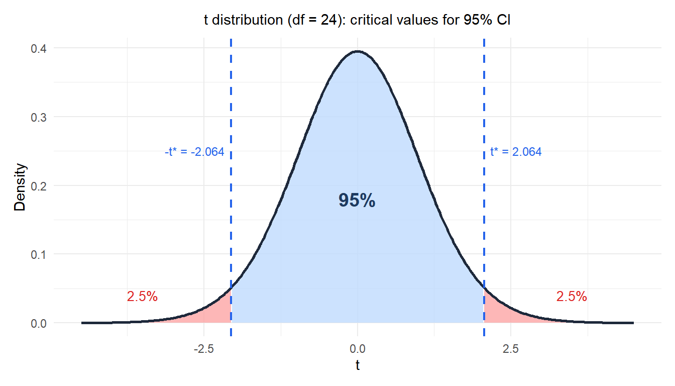
Example 1: hospital length of stay
A hospital records the length of stay (days) for a random sample of 25 patients: \(\bar{x} = 6.4\) days, \(S = 3.1\) days. Construct a 95% CI for the population mean.
Step 1: identify the ingredients.
\[n = 25, \quad \bar{x} = 6.4, \quad S = 3.1, \quad \alpha = 0.05\]
Step 2: find the critical value.
\[t_{0.025,\; 24} = 2.064\]
Step 3: compute the standard error and margin of error.
\[\text{SE} = \frac{3.1}{\sqrt{25}} = \frac{3.1}{5} = 0.62, \qquad \text{ME} = 2.064 \times 0.62 = 1.28\]
Step 4: build the interval.
\[\text{CI} = 6.4 \pm 1.28 = [5.12,\; 7.68] \text{ days}\]
We are 95% confident that the true average length of stay is between 5.1 and 7.7 days.
Example 2: manufacturing process
A factory samples 60 components and measures their tensile strength. Results: \(\bar{x} = 248.3\) MPa, \(S = 12.7\) MPa. Construct a 99% CI.
\[t_{0.005,\; 59} \approx 2.662\]
\[\text{ME} = 2.662 \times \frac{12.7}{\sqrt{60}} = 2.662 \times 1.640 = 4.37 \text{ MPa}\]
\[\text{CI} = 248.3 \pm 4.37 = [243.9,\; 252.7] \text{ MPa}\]
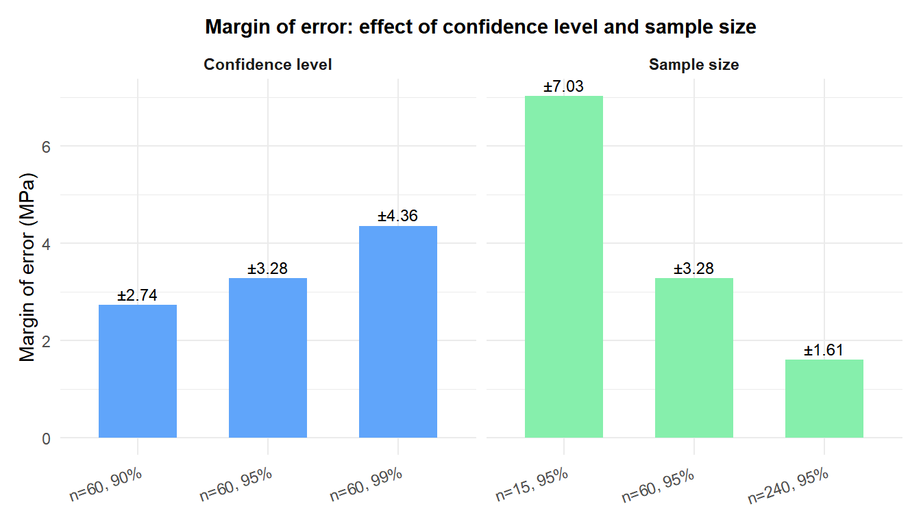
Using the same data (\(S = 12.7\) MPa):
| Configuration | \(t^*\) | SE | Margin of error |
|---|---|---|---|
| \(n=60\), 90% | 1.671 | 1.64 | ±2.74 MPa |
| \(n=60\), 95% | 2.001 | 1.64 | ±3.28 MPa |
| \(n=60\), 99% | 2.662 | 1.64 | ±4.37 MPa |
| \(n=15\), 95% | 2.145 | 3.28 | ±7.04 MPa |
| \(n=60\), 95% | 2.001 | 1.64 | ±3.28 MPa |
| \(n=240\), 95% | 1.970 | 0.82 | ±1.62 MPa |
Quadrupling \(n\) from 15 to 60 halves the margin of error. Going from 95% to 99% confidence adds about 1 MPa.
💡 Practical guidance
- Report the CI alongside the point estimate: “\(\bar{x} = 248.3\) MPa (95% CI: 243.9 to 252.7 MPa)”.
- To plan sample size: decide the maximum acceptable margin of error \(d\), then solve \(n \approx (t^* S / d)^2\).
- If data is heavily skewed and \(n\) is small, the \(t\) CI may be unreliable. Consider a log-transformation or bootstrap CI.
- One-sided CIs (lower bound only or upper bound only) use \(t_{\alpha,\, n-1}\) instead of \(t_{\alpha/2,\, n-1}\).

