Pareto distribution
The Pareto distribution models phenomena where a small fraction of observations accounts for most of the total effect. It is the mathematical foundation of the 80/20 rule and describes wealth, city sizes, earthquake magnitudes, and internet traffic, in contexts where extreme events are far more common than the normal distribution would predict.
Definition
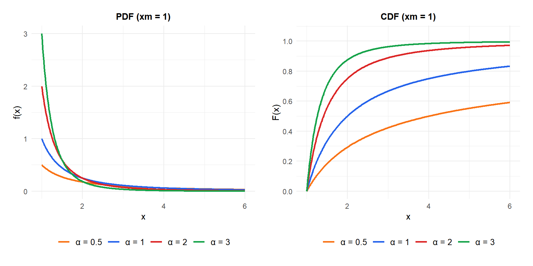
A random variable \(X\) follows a Pareto distribution with scale parameter \(x_m > 0\) (minimum possible value) and shape parameter \(\alpha > 0\) (tail index), written \(X \sim \text{Pareto}(x_m, \alpha)\), if:
\[f(x) = \frac{\alpha\, x_m^\alpha}{x^{\alpha+1}}, \quad x \geq x_m\]
The CDF has a clean closed form:
\[F(x) = 1 - \left(\frac{x_m}{x}\right)^\alpha, \quad x \geq x_m\]
The survival function \(P(X > x) = (x_m/x)^\alpha\) decays as a power law: halving \(\alpha\) squares the probability of exceeding any threshold. This is what makes the Pareto “heavy-tailed”: the tail decays much more slowly than the exponential \(e^{-\lambda x}\).
Properties
For \(X \sim \text{Pareto}(x_m, \alpha)\):
- Expected Value (Mean)
\[E(X) = \frac{\alpha\, x_m}{\alpha - 1}, \quad \text{only defined for } \alpha > 1\]
For \(\alpha \leq 1\), the mean is infinite.
- Variance
\[\text{Var}(X) = \frac{\alpha\, x_m^2}{(\alpha-1)^2(\alpha-2)}, \quad \text{only defined for } \alpha > 2\]
For \(1 < \alpha \leq 2\), the mean exists but the variance is infinite.
- Skewness
\[\text{Skewness} = \frac{2(1+\alpha)}{\alpha - 3}\sqrt{\frac{\alpha-2}{\alpha}}, \quad \text{for } \alpha > 3\]
Undefined for \(\alpha \leq 3\). Always positive (right-skewed).
- Kurtosis
\[g_2 = \frac{6(\alpha^3 + \alpha^2 - 6\alpha - 2)}{\alpha(\alpha-3)(\alpha-4)}, \quad \text{for } \alpha > 4\]
- Median
\[\text{Median} = x_m \cdot 2^{1/\alpha}\]
- Mode
\[\text{Mode} = x_m\]
The distribution is always decreasing: the most likely value is the minimum \(x_m\).
- Quantile Function
\[Q(p) = \frac{x_m}{(1-p)^{1/\alpha}}\]
⚠️ Mean and variance may not exist
The Pareto distribution is unusual in that its moments can fail to exist:
- \(\alpha \leq 1\): the mean is infinite. Averages computed from samples will grow without bound as \(n\) increases.
- \(1 < \alpha \leq 2\): the mean exists but the variance is infinite. The sample variance will keep growing with sample size.
- \(\alpha > 2\): both mean and variance exist.
In practice, \(\alpha\) for wealth distributions is often estimated around 1.5, meaning wealth has a finite mean but infinite variance. This is why “the average wealth” can be a misleading statistic.
The 80/20 rule
The Pareto principle states that roughly 80% of effects come from 20% of causes. This is not a law of nature but a consequence of the Pareto distribution when \(\alpha = \log(5)/\log(4) \approx 1.161\).
More generally, the fraction of the population \(p\) that accounts for fraction \(F\) of the total (for a Pareto-distributed quantity with \(\alpha > 1\)) is:
\[F = 1 - \left(\frac{x_m}{Q(1-p)}\right)^{\alpha-1} = 1 - (1-p)^{(\alpha-1)/\alpha}\]
For \(\alpha = 1.161\) (the exact Pareto exponent for the 80/20 rule):
- The top 20% of earners hold 80% of total income.
- The top 4% hold 64% of total income (\(0.2^2 = 0.04\), \(0.8^2 = 0.64\)).
- The top 1% hold about 55% of total income.
These numbers are not coincidences: they follow directly from the power-law structure of the Pareto distribution.
Step-by-step example
Insurance claims above a minimum threshold of 10,000 USD follow a Pareto distribution with \(x_m = 10{,}000\) and \(\alpha = 2.5\).
Expected claim size:
\[E(X) = \frac{2.5 \times 10{,}000}{2.5 - 1} = \frac{25{,}000}{1.5} \approx 16{,}667 \text{ USD}\]
Probability of a claim exceeding 50,000 USD:
\[P(X > 50{,}000) = \left(\frac{10{,}000}{50{,}000}\right)^{2.5} = (0.2)^{2.5} \approx 0.0179\]
About 1.8% of claims exceed 50,000 USD.
90th percentile (claims that only 10% of policies exceed):
\[Q(0.90) = \frac{10{,}000}{(1-0.90)^{1/2.5}} = \frac{10{,}000}{0.1^{0.4}} \approx \frac{10{,}000}{0.251} \approx 39{,}800 \text{ USD}\]
Variance:
\[\text{Var}(X) = \frac{2.5 \times 10{,}000^2}{(1.5)^2 \times (0.5)} = \frac{250{,}000{,}000}{1.125} \approx 222{,}222{,}222 \text{ USD}^2\]
Standard deviation \(\approx 14{,}907\) USD, which is almost as large as the mean.
⚠️ Power-law tails vs exponential tails
The key difference between the Pareto and distributions like the exponential or normal is how fast the tail decays:
- Exponential tail: \(P(X > x) = e^{-\lambda x}\). Decays extremely fast. Doubling \(x\) squares the tail probability only roughly.
- Power-law tail: \(P(X > x) = (x_m/x)^\alpha\). Decays slowly. An earthquake 10 times larger is only \(10^\alpha\) times rarer, not exponentially rarer.
This is why 100-year floods, billion-dollar insurance losses, and mega-viral social media posts exist: exponential-tailed models would predict them as essentially impossible, but power-law models assign them non-negligible probability.
💡 Relationship with other distributions
- Exponential: the Pareto is the continuous analogue of the geometric in the sense of memorylessness, but with a power-law rather than exponential tail.
- Lomax (Pareto Type II): \(Y = X - x_m\) where \(X \sim \text{Pareto}(x_m, \alpha)\) gives a Lomax distribution starting at 0.
- Log-uniform: if \(\ln(X)\) is uniform on \((\ln x_m, \infty)\), \(X\) is Pareto.
- Generalized Pareto: used in extreme value theory to model exceedances above a threshold, generalizing the standard Pareto.

