VAR model
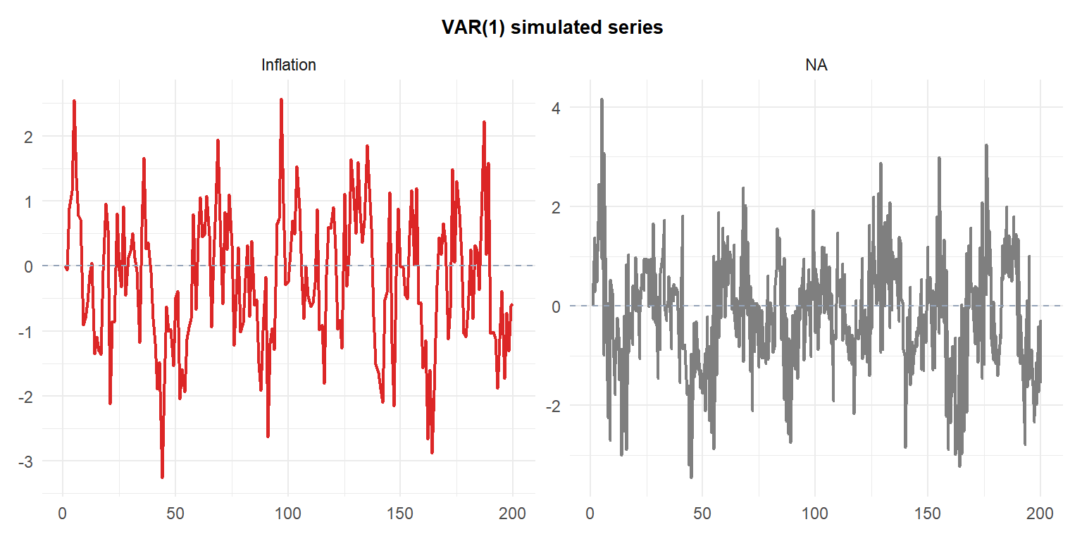
A VAR (Vector Autoregression) models multiple time series simultaneously, allowing each variable to depend on its own lags and the lags of all other variables. It is the standard framework for analyzing interdependencies between macroeconomic or financial series without imposing strong prior restrictions on which variables affect which.
From univariate to multivariate
ARIMA models one series at a time. But many series interact: GDP affects inflation, interest rates affect exchange rates, oil prices affect industrial production. Modeling each series separately ignores these cross-variable dynamics and produces suboptimal forecasts.
VAR treats all variables symmetrically: every variable can potentially affect every other variable. This makes it useful for:
- Forecasting: joint forecasts that respect cross-variable correlations.
- Structural analysis: impulse response functions show how a shock in one variable propagates through the system.
- Granger causality: testing whether one series helps predict another.
Definition
A VAR(\(p\)) model for a \(k\)-dimensional vector \(\mathbf{y}_t = (y_{1t}, y_{2t}, \ldots, y_{kt})'\):
\[\mathbf{y}_t = \mathbf{c} + \mathbf{A}_1 \mathbf{y}_{t-1} + \mathbf{A}_2 \mathbf{y}_{t-2} + \cdots + \mathbf{A}_p \mathbf{y}_{t-p} + \boldsymbol{\varepsilon}_t\]
\[\boldsymbol{\varepsilon}_t \sim \text{WN}(\mathbf{0}, \boldsymbol{\Sigma})\]
where: - \(\mathbf{c}\): \(k \times 1\) vector of intercepts. - \(\mathbf{A}_i\): \(k \times k\) coefficient matrices at lag \(i\). - \(\boldsymbol{\Sigma}\): \(k \times k\) positive definite covariance matrix of the innovations.
Total parameters: \(k^2 p + k\) (plus the \(k(k+1)/2\) unique elements of \(\boldsymbol{\Sigma}\)). For \(k=3\), \(p=2\): already 21 coefficients. For \(k=5\), \(p=4\): 105 coefficients. Parameter proliferation is the main practical constraint.
Each equation is a regression of \(y_{it}\) on all \(p\) lags of all \(k\) variables. The system can be estimated equation by equation by OLS (efficient when all equations have the same regressors).
Stationarity condition
A VAR(\(p\)) is stationary if all eigenvalues of the companion matrix have modulus less than 1. For VAR(1), this reduces to: all eigenvalues of \(\mathbf{A}_1\) lie inside the unit circle.
Equivalently, all roots of \(\det(\mathbf{I}_k - \mathbf{A}_1 z - \cdots - \mathbf{A}_p z^p) = 0\) must lie outside the unit circle.
⚠️ Non-stationary series in a VAR require cointegration analysis
If any series has a unit root, fitting a VAR in levels produces spurious results. Two options:
- Difference all series before fitting: produces a stationary VAR but loses long-run information.
- VECM (Vector Error Correction Model): if the non-stationary series are cointegrated (share a common stochastic trend), fit a VECM that combines differenced dynamics with an error correction term representing the long-run relationship. This is the preferred approach for series like GDP and consumption, or prices across markets.
Always test for unit roots (ADF/KPSS) and cointegration (Johansen test) before choosing between VAR in levels, VAR in differences, or VECM.
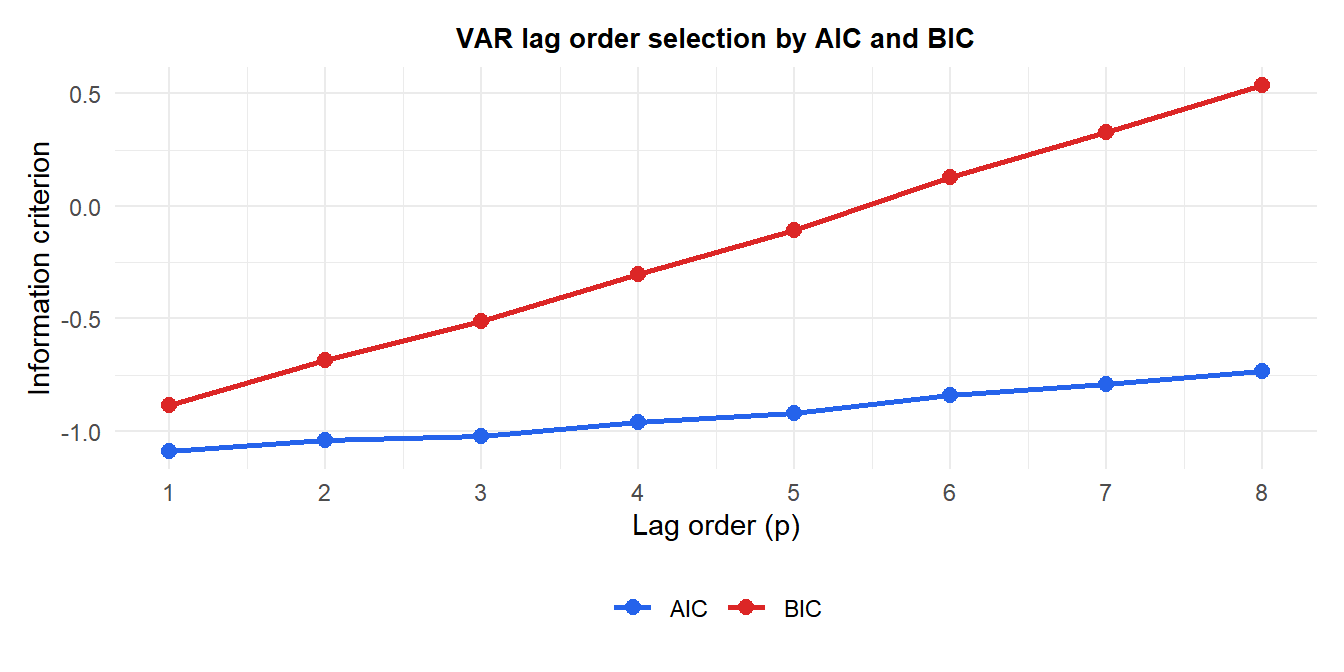
Lag order selection
The order \(p\) is selected by information criteria computed across the full system:
\[\text{AIC} = \log|\hat{\boldsymbol{\Sigma}}| + \frac{2k^2p}{T}, \qquad \text{BIC} = \log|\hat{\boldsymbol{\Sigma}}| + \frac{\log(T) k^2 p}{T}\]
Impulse response functions (IRF)
The most important tool in VAR analysis. An IRF traces the dynamic response of each variable to a one-unit shock in one variable, holding all other shocks at zero.
For an orthogonalized IRF (using Cholesky decomposition of \(\boldsymbol{\Sigma}\)), the ordering of variables matters: the first variable is assumed to have contemporaneous effects on all others, but not vice versa. This ordering should reflect economic theory.
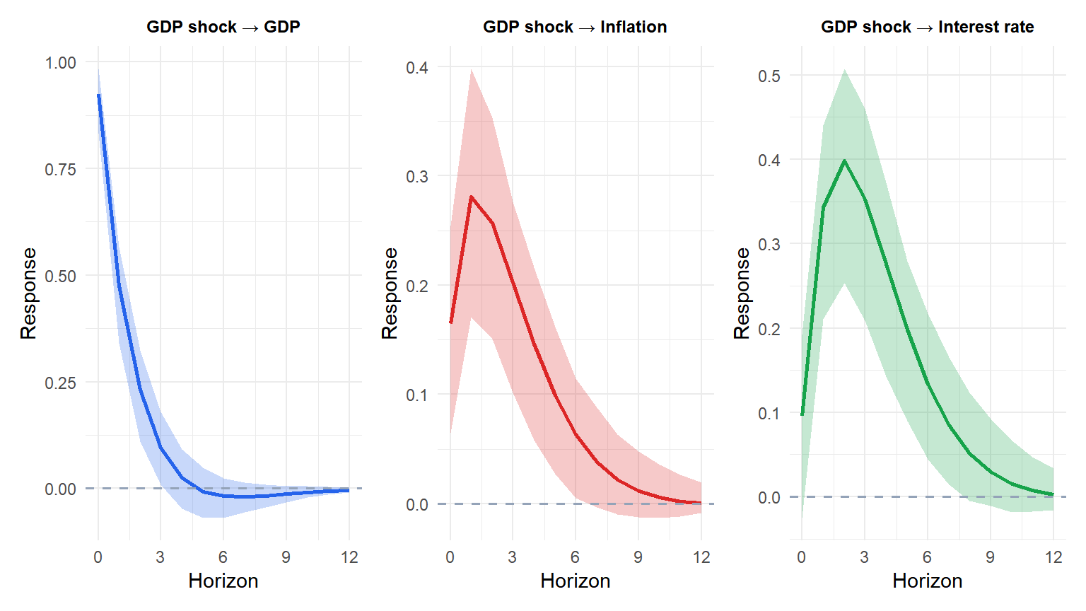
A positive shock to GDP (y1) raises GDP itself (persistent but decaying), passes through to inflation (positive response with a lag), and eventually pushes up the interest rate. The shaded bands are 95% bootstrap confidence intervals.
Forecast error variance decomposition (FEVD)
FEVD quantifies what fraction of the \(h\)-step forecast error variance of variable \(i\) is attributable to shocks in variable \(j\). It answers: “how important is variable \(j\) for explaining the variability of variable \(i\) at horizon \(h\)?”
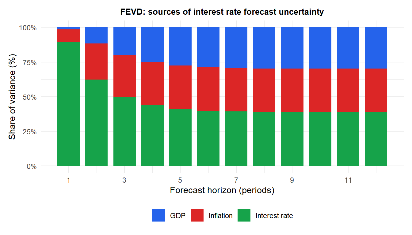
At short horizons, GDP uncertainty is mainly driven by its own shocks. As the horizon extends, inflation and interest rate shocks contribute more, reflecting the cross-variable propagation captured by the VAR.
Granger causality
Variable \(x\) Granger-causes \(y\) if past values of \(x\) help predict \(y\) beyond what past values of \(y\) alone can predict. In a VAR framework, this is tested by checking whether the coefficients on \(x\) lags in the \(y\) equation are jointly zero:
\[H_0: \mathbf{A}_{1,yx} = \mathbf{A}_{2,yx} = \cdots = \mathbf{A}_{p,yx} = \mathbf{0}\]
using a Wald test (\(\chi^2\) with \(kp\) degrees of freedom).
⚠️ Granger causality is not economic causality
Granger causality is a statement about predictability, not about causal mechanisms. If \(x\) Granger-causes \(y\), it means \(x\) contains predictive information about \(y\). It does not mean that changing \(x\) will change \(y\): there could be a common driver causing both, or the relationship could be coincidental.
For causal inference from observational VAR data, structural identification (via economic theory, sign restrictions, or external instruments) is required. Granger causality is a preliminary screening tool, not evidence of economic causation.
💡 VAR in R
library(vars)

# Fit VAR(p)
VARselect(y, lag.max = 8)   # choose p by AIC/BIC
fit <- VAR(y, p = 2, type = "const")
summary(fit)

# Impulse response functions
irf(fit, impulse = "gdp", response = "inflation",
    n.ahead = 12, boot = TRUE)

# Forecast error variance decomposition
fevd(fit, n.ahead = 12)

# Granger causality test
causality(fit, cause = "gdp")

# Forecast
predict(fit, n.ahead = 8)
