Stationarity in time series
A stationary time series has constant mean, constant variance, and autocorrelations that depend only on the lag, not on time. Most time series models assume stationarity. Detecting and correcting non-stationarity is the essential first step before fitting AR, MA, ARIMA, or any other model.
Formal definition
A time series \(\{y_t\}\) is weakly stationary (or covariance-stationary) if:
\[E[y_t] = \mu \quad \forall t \qquad \text{(constant mean)}\] \[\text{Var}(y_t) = \sigma^2 < \infty \quad \forall t \qquad \text{(constant variance)}\] \[\text{Cov}(y_t, y_{t+k}) = \gamma(k) \quad \forall t \qquad \text{(autocovariance depends only on lag } k \text{)}\]
Strict stationarity requires the entire joint distribution of \((y_t, y_{t+1}, \ldots, y_{t+k})\) to be invariant to time shifts. For practical purposes, weak stationarity is sufficient.
A series that is not stationary is called non-stationary or integrated. The most common form of non-stationarity in economic and financial data is the unit root: a stochastic trend that causes the series to wander without mean-reverting.
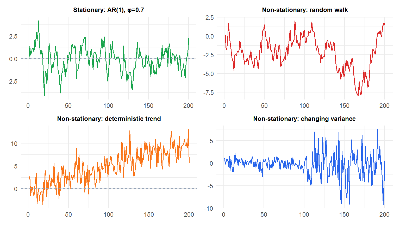
The stationary series (green) fluctuates around a constant mean. The random walk (red) drifts without bound. The trended series (orange) has a rising mean. The heteroscedastic series (blue) has variance that changes mid-sample.
Unit roots and random walks
The most important source of non-stationarity in practice is the unit root. An AR(1) process:
\[y_t = \phi y_{t-1} + \varepsilon_t\]
is stationary when \(|\phi| < 1\) (the series reverts to its mean). When \(\phi = 1\), it becomes a random walk:
\[y_t = y_{t-1} + \varepsilon_t \implies y_t = y_0 + \sum_{s=1}^t \varepsilon_s\]
The variance of a random walk grows without bound: \(\text{Var}(y_t) = t\sigma^2\). Shocks are permanent: they never dissipate. This is why testing for \(\phi = 1\) (a unit root) is central to time series analysis.
Testing for stationarity
Augmented Dickey-Fuller (ADF) test
Tests \(H_0\): the series has a unit root (non-stationary) vs \(H_1\): the series is stationary. The test fits the regression:
\[\Delta y_t = \alpha + \beta t + \gamma y_{t-1} + \sum_{j=1}^p \delta_j \Delta y_{t-j} + \varepsilon_t\]
and tests \(H_0: \gamma = 0\) (unit root present). Reject \(H_0\) if the t-statistic for \(\gamma\) is sufficiently negative (critical values are non-standard, not from the normal distribution).
The number of lags \(p\) is chosen to remove autocorrelation from the residuals (typically by AIC or BIC).
KPSS test (Kwiatkowski-Phillips-Schmidt-Shin)
Tests the opposite: \(H_0\): the series is stationary vs \(H_1\): the series has a unit root. Large values of the KPSS statistic reject stationarity.
⚠️ ADF and KPSS have opposite null hypotheses - do not confuse them
The most common mistake: treating both tests as if they test the same thing.
- ADF: \(H_0\) = unit root (non-stationary). A large p-value means you fail to reject non-stationarity. A small p-value means you reject the unit root, supporting stationarity.
- KPSS: \(H_0\) = stationarity. A large p-value means you fail to reject stationarity. A small p-value means you reject stationarity.
Interpreting: “ADF p-value = 0.60, therefore the series is stationary” is wrong. A p-value of 0.60 means you failed to reject the unit root, i.e., you have no evidence against non-stationarity.
Use both tests together. If ADF rejects the unit root AND KPSS does not reject stationarity: strong evidence for stationarity. If both fail to agree: investigate further.
Phillips-Perron (PP) test
A nonparametric alternative to ADF. Same \(H_0\) (unit root), but uses a different correction for autocorrelation in the residuals instead of adding lagged differences. Tends to be more robust to heteroscedasticity.
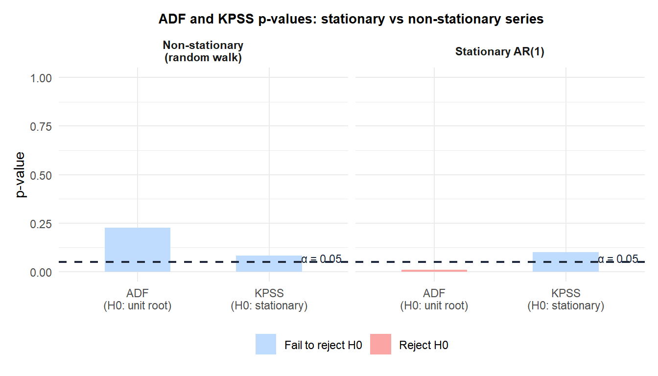
For the stationary AR(1): ADF rejects the unit root (red, \(p < 0.05\)) and KPSS fails to reject stationarity (blue, \(p > 0.05\)). Both agree: stationary. For the random walk: ADF fails to reject the unit root (blue) and KPSS rejects stationarity (red). Both agree: non-stationary.
Transformations to achieve stationarity
Differencing
The standard remedy for a unit root. First difference removes a linear stochastic trend:
\[\Delta y_t = y_t - y_{t-1}\]
A series that becomes stationary after \(d\) differences is called integrated of order \(d\), denoted \(I(d)\). Most economic series are \(I(1)\): one difference suffices.
Log transformation
Stabilizes variance that grows proportionally with the level (common in prices, GDP, sales). \(\log(y_t)\) converts multiplicative seasonality to additive and makes the series more symmetric.
Box-Cox transformation
A family of power transformations parameterized by \(\lambda\):
\[y_t^{(\lambda)} = \begin{cases} (y_t^\lambda - 1)/\lambda & \lambda \neq 0 \\ \log(y_t) & \lambda = 0 \end{cases}\]
The optimal \(\lambda\) is estimated from the data. \(\lambda = 1\) is no transformation; \(\lambda = 0\) is log; \(\lambda = 0.5\) is square root.
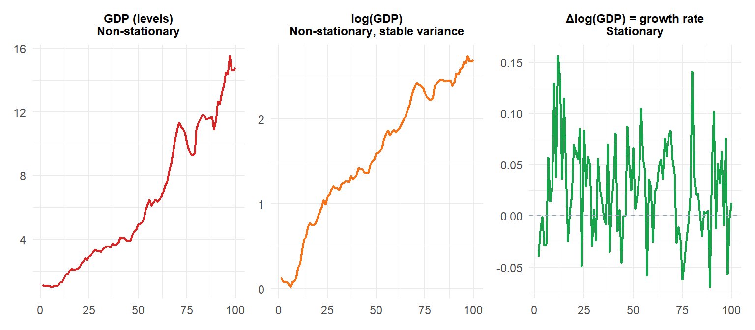
GDP in levels (red) is non-stationary with growing variance. After log (orange), variance stabilizes but the trend remains. After first-differencing log(GDP) (green), the series becomes stationary: it represents the GDP growth rate, fluctuating around a constant mean.
How many differences?
Apply the ADF test after each differencing step until stationarity is achieved. For most economic series, \(d=1\) suffices. Over-differencing (applying more differences than needed) makes the series harder to model and should be avoided.
A practical rule: if the ADF test on the original series fails to reject the unit root, difference once and test again. If the ADF on \(\Delta y_t\) rejects the unit root, \(d=1\) is appropriate.
💡 Stationarity tests in R
library(tseries)

# ADF test (H0: unit root)
adf.test(y)
adf.test(diff(y))   # after first differencing

# KPSS test (H0: stationary)
kpss.test(y)

# Phillips-Perron test (H0: unit root)
pp.test(y)

# Automatic differencing order selection
library(forecast)
ndiffs(y)     # number of regular differences needed
nsdiffs(y)    # number of seasonal differences needed
