Moving average model (MA)
A moving average model of order \(q\), MA(\(q\)), expresses the current value as a linear combination of the current and \(q\) past white noise errors. Unlike AR models, MA models are always stationary regardless of the parameter values. The invertibility condition determines whether the model has a useful AR representation.
Definition
\[y_t = \mu + \varepsilon_t + \theta_1 \varepsilon_{t-1} + \theta_2 \varepsilon_{t-2} + \cdots + \theta_q \varepsilon_{t-q}\]
where \(\varepsilon_t \sim \text{WN}(0, \sigma^2)\). Using the lag operator:
\[y_t - \mu = \Theta(L)\,\varepsilon_t, \qquad \Theta(L) = 1 + \theta_1 L + \theta_2 L^2 + \cdots + \theta_q L^q\]
The \(\theta_i\) measure how past shocks propagate into current values. A positive \(\theta_1\) means a positive shock today raises tomorrow’s value; negative \(\theta_1\) creates an overshooting correction.
MA processes are always stationary
For any finite \(q\) and any values of \(\theta_1, \ldots, \theta_q\):
\[E[y_t] = \mu, \quad \text{Var}(y_t) = \sigma^2(1 + \theta_1^2 + \cdots + \theta_q^2)\]
Both are constants, independent of \(t\). The autocovariance:
\[\gamma_k = \begin{cases} \sigma^2 \sum_{j=0}^{q-k} \theta_j \theta_{j+k} & k = 1, 2, \ldots, q \\ 0 & k > q \end{cases}\]
depends only on lag \(k\), not on \(t\). Therefore every MA(\(q\)) is weakly stationary. This contrasts with AR models, where stationarity requires the root condition \(|\phi_1| < 1\) for AR(1), etc.
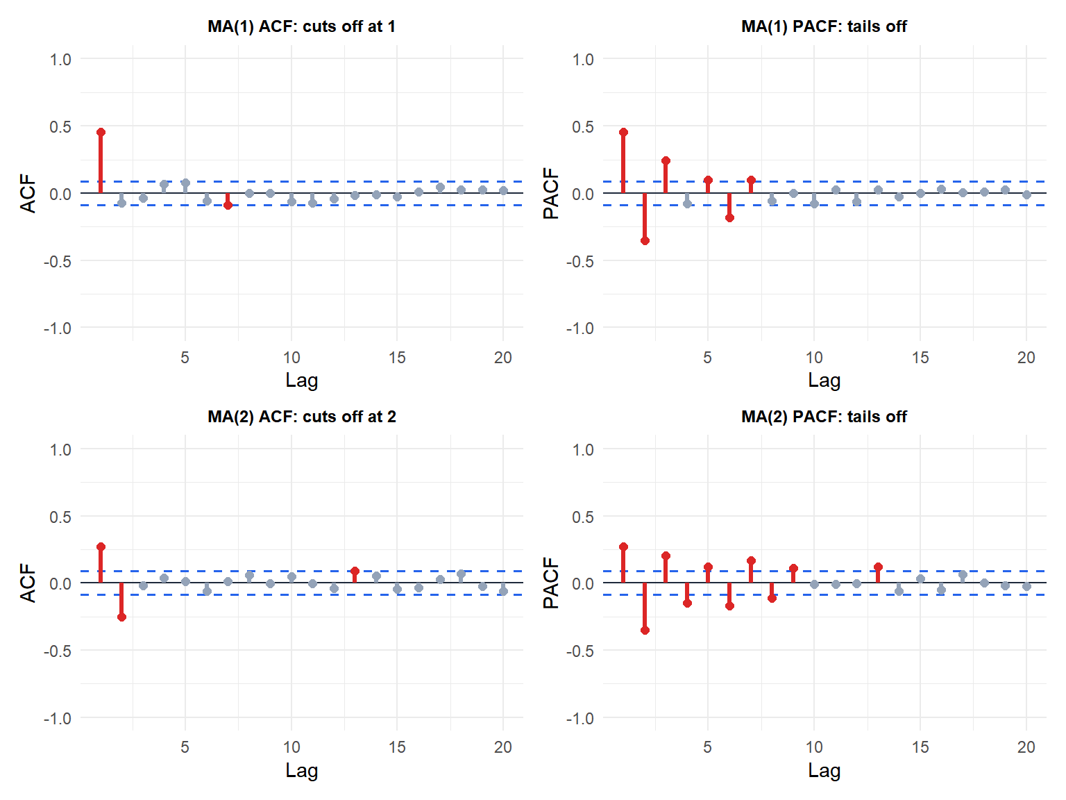
ACF and PACF of MA processes
The theoretical ACF of MA(\(q\)) cuts off exactly at lag \(q\):
\[\rho_k = \begin{cases} \dfrac{\sum_{j=0}^{q-k} \theta_j \theta_{j+k}}{1 + \theta_1^2 + \cdots + \theta_q^2} & k = 1, \ldots, q \\ 0 & k > q \end{cases}\]
The PACF tails off geometrically (or with damped oscillations). This is the mirror image of the AR pattern, and the key identifier for MA models.
Invertibility
An MA(\(q\)) process is invertible if all roots of \(\Theta(z) = 1 + \theta_1 z + \cdots + \theta_q z^q = 0\) lie outside the unit circle \(|z| > 1\).
Invertibility means the MA process can be written as an AR(\(\infty\)):
\[y_t = \sum_{j=1}^\infty \pi_j y_{t-j} + \varepsilon_t\]
where the \(\pi_j\) coefficients decay to zero. This AR(\(\infty\)) representation is what makes the model useful: it allows estimation by expressing current errors in terms of observable past values.
For MA(1): \(y_t = \varepsilon_t + \theta_1 \varepsilon_{t-1}\) is invertible iff \(|\theta_1| < 1\). The AR(\(\infty\)) representation is:
\[\varepsilon_t = y_t - \theta_1 y_{t-1} + \theta_1^2 y_{t-2} - \theta_1^3 y_{t-3} + \cdots = \sum_{j=0}^\infty (-\theta_1)^j y_{t-j}\]
which converges only when \(|\theta_1| < 1\).
⚠️ Non-invertible MA models are not identifiable
For any non-invertible MA(\(q\)) with parameter \(\theta_1\), there exists an invertible MA(\(q\)) with parameter \(1/\theta_1\) that has the same ACF. The two models are observationally equivalent from the ACF alone.
Example: MA(1) with \(\theta_1 = 2\) and MA(1) with \(\theta_1 = 0.5\) have the same autocorrelation \(\rho_1 = \theta_1/(1+\theta_1^2)\). By convention, we always choose the invertible solution (\(|\theta_1| < 1\)). Software enforces this automatically.
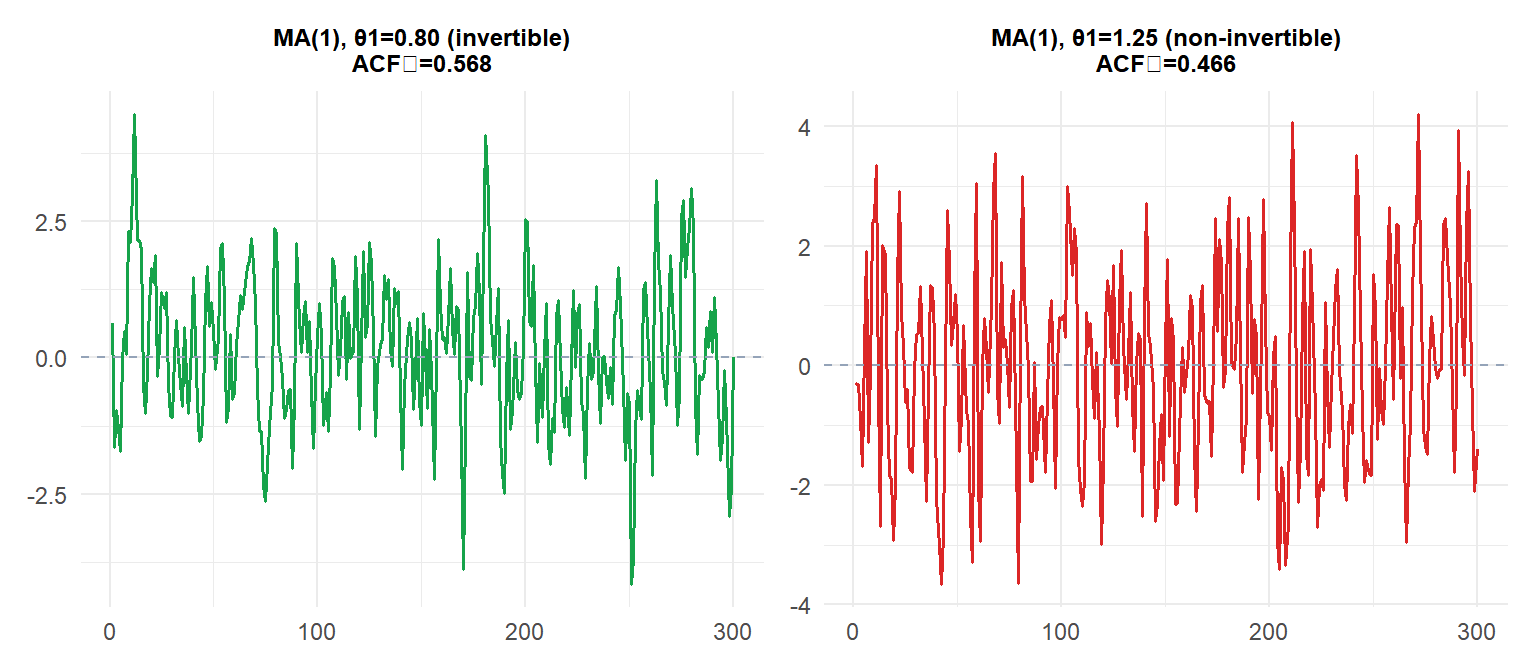
Both series have nearly identical ACF at lag 1, confirming the observational equivalence. By convention the invertible solution (\(|\theta_1| < 1\)) is always chosen.
Example: MA(1) for stock returns
Daily excess returns of a stock often show a small negative MA(1) component: a day of above-average returns is slightly followed by a day of below-average returns (bid-ask bounce effect).
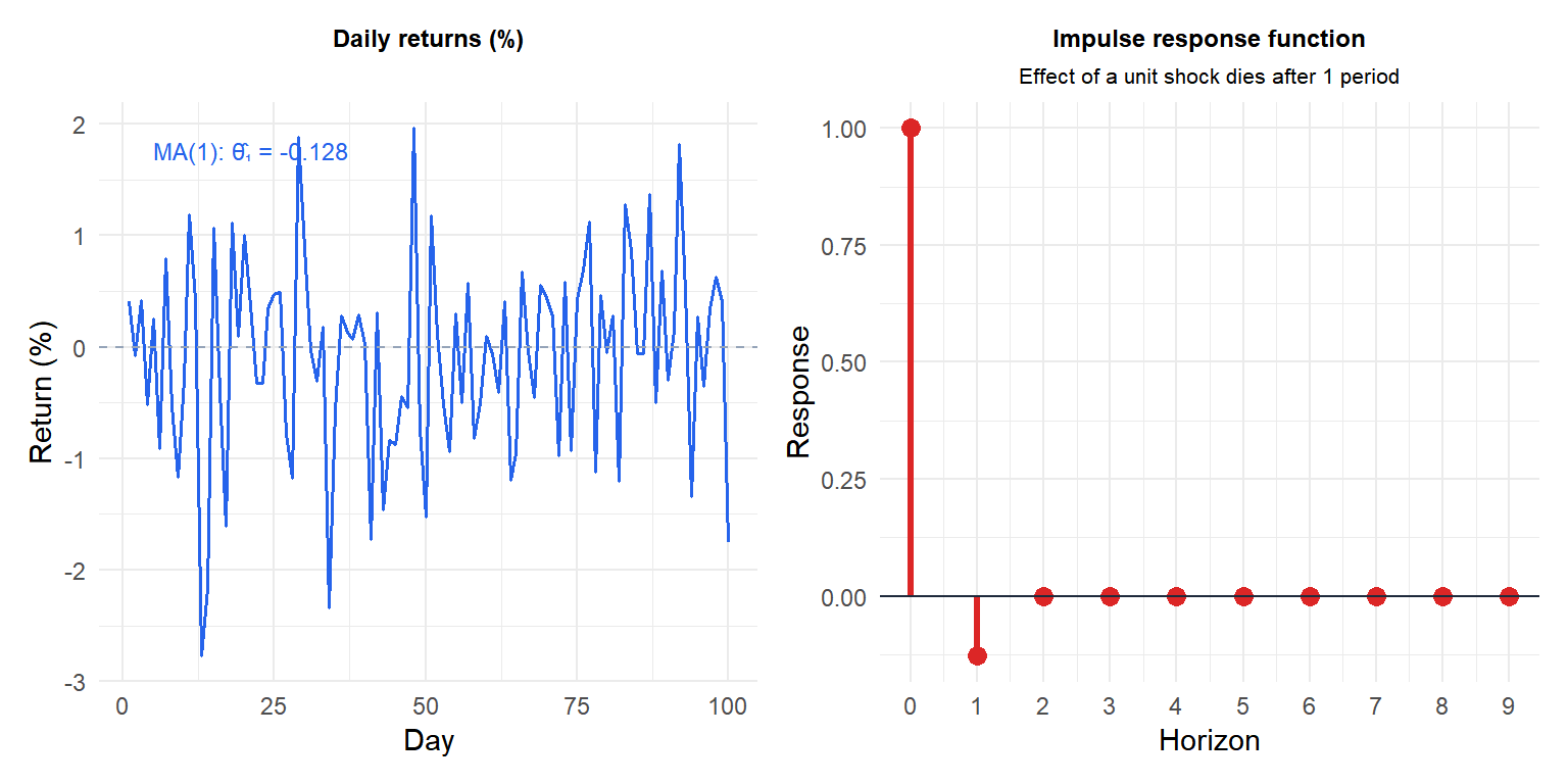
The impulse response function (IRF) shows the effect of a unit shock on current and future values. For MA(\(q\)), the response is exactly zero after \(q\) periods: shocks have finite memory. This contrasts with AR models, where shocks decay geometrically but never fully disappear.
MA vs AR: key differences
| Property | AR(\(p\)) | MA(\(q\)) |
|---|---|---|
| Always stationary | No | Yes |
| Invertibility required | Always | Only for AR(\(\infty\)) representation |
| ACF | Tails off | Cuts off at \(q\) |
| PACF | Cuts off at \(p\) | Tails off |
| Memory of shocks | Infinite (geometric decay) | Finite (\(q\) periods) |
| Estimation | OLS, Yule-Walker, MLE | MLE (non-linear) |
💡 Fitting MA models in R
# Fit MA(1)
arima(y, order = c(0, 0, 1))

# Fit MA(2)
arima(y, order = c(0, 0, 2))

# Check invertibility: roots should be outside unit circle
fit <- arima(y, order = c(0, 0, 1))
polyroot(c(1, coef(fit)["ma1"]))  # modulus should be > 1
Unlike AR models, MA parameters cannot be estimated by OLS because the past errors \(\varepsilon_{t-j}\) are unobservable. MLE is the standard method.

