GARCH model
GARCH (Generalized Autoregressive Conditional Heteroscedasticity) models the conditional variance of a time series as a function of past squared errors and past variances. It captures the most pervasive stylized fact of financial returns: volatility clustering, where large moves tend to be followed by large moves regardless of direction.
Motivation: volatility clustering
Financial return series have approximately zero autocorrelation in levels but strong autocorrelation in squared returns. This means:
- The mean is hard to predict from past returns (consistent with market efficiency).
- The variance is predictable: high-volatility periods cluster together.
ARIMA models the conditional mean but assumes constant variance. GARCH models the conditional variance, which ARIMA leaves unexplained.
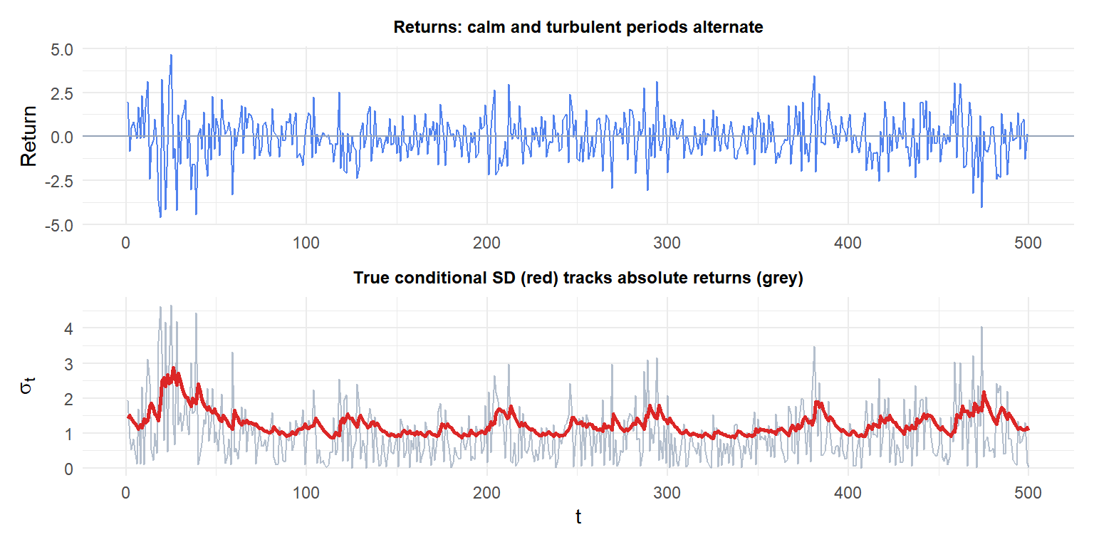
Large swings in returns (blue) coincide with high conditional volatility (red). Quiet periods have low conditional volatility. ARIMA would assign constant variance to all periods.
ARCH: the precursor
Robert Engle (1982, Nobel Prize 2003) introduced ARCH(\(q\)) (AutoRegressive Conditional Heteroscedasticity):
\[r_t = \mu_t + \varepsilon_t, \qquad \varepsilon_t = \sigma_t z_t, \quad z_t \sim \text{i.i.d.}(0,1)\]
\[\sigma_t^2 = \omega + \alpha_1 \varepsilon_{t-1}^2 + \alpha_2 \varepsilon_{t-2}^2 + \cdots + \alpha_q \varepsilon_{t-q}^2\]
The conditional variance \(\sigma_t^2\) is a linear function of \(q\) past squared residuals. A large shock at \(t-1\) increases \(\sigma_t^2\), producing volatility clustering.
Limitation: capturing long memory in volatility requires large \(q\), estimating many \(\alpha_i\) parameters. Bollerslev (1986) generalized this to GARCH.
GARCH(\(p,q\))
Generalized ARCH adds \(p\) lagged conditional variances to the equation:
\[\sigma_t^2 = \omega + \sum_{i=1}^q \alpha_i \varepsilon_{t-i}^2 + \sum_{j=1}^p \beta_j \sigma_{t-j}^2\]
The most common specification is GARCH(1,1):
\[\sigma_t^2 = \omega + \alpha_1 \varepsilon_{t-1}^2 + \beta_1 \sigma_{t-1}^2\]
- \(\omega > 0\): long-run variance floor.
- \(\alpha_1 \geq 0\): reaction coefficient. How much a large shock increases next period’s variance.
- \(\beta_1 \geq 0\): persistence coefficient. How slowly volatility decays after a shock.
- \(\alpha_1 + \beta_1\): total persistence. Must be \(< 1\) for covariance stationarity.
The unconditional (long-run) variance is:
\[\sigma^2 = \frac{\omega}{1 - \alpha_1 - \beta_1}\]
GARCH(1,1) is sufficient for most financial series. The \(\beta_1\) term captures the slow decay of volatility without needing many \(\alpha_i\) lags.
Stationarity and positivity conditions
For GARCH(1,1) to be well-defined:
| Condition | Requirement |
|---|---|
| Positivity of \(\sigma_t^2\) | \(\omega > 0\), \(\alpha_1 \geq 0\), \(\beta_1 \geq 0\) |
| Covariance stationarity | \(\alpha_1 + \beta_1 < 1\) |
| Finite fourth moment | \(3\alpha_1^2 + 2\alpha_1\beta_1 + \beta_1^2 < 1\) (for Gaussian \(z_t\)) |
When \(\alpha_1 + \beta_1 = 1\), the process is IGARCH (integrated GARCH): shocks to variance are permanent (infinite persistence). This is sometimes observed in very high-frequency financial data.
Testing for ARCH effects
Before fitting GARCH, verify that ARCH effects are present using the Ljung-Box test on squared residuals or the ARCH-LM test:
- Fit an ARIMA model to the return series to remove the conditional mean.
- Extract residuals \(\hat{\varepsilon}_t\).
- Test whether \(\hat{\varepsilon}_t^2\) is autocorrelated.
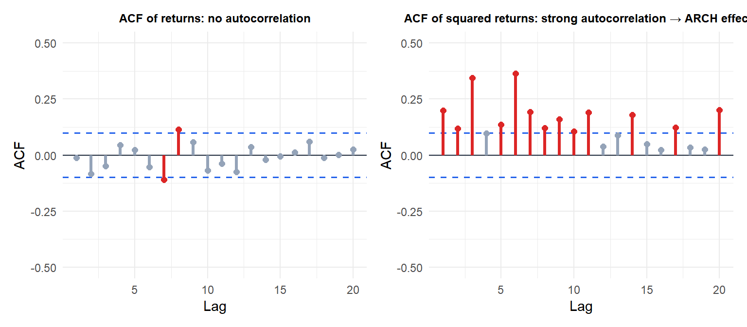
Returns (left) show no significant autocorrelation. Squared returns (right) show strong autocorrelation: evidence of ARCH effects. GARCH is appropriate.
Example: fitting GARCH(1,1) to stock returns
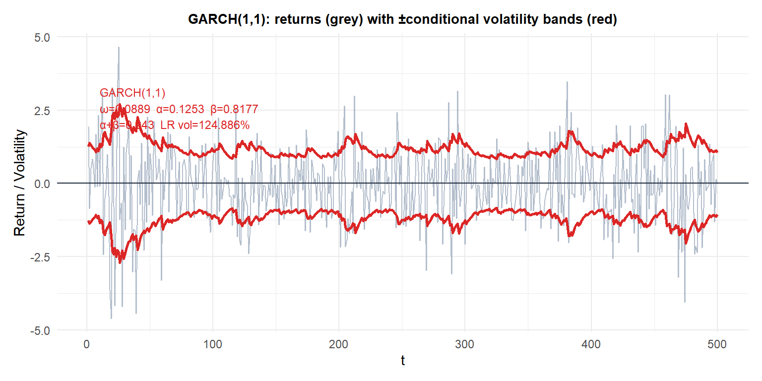
The red bands show \(\pm\hat{\sigma}_t\): they widen during turbulent periods and narrow during calm ones. The persistence \(\alpha + \beta \approx 0.95\) is typical of daily financial returns: volatility shocks take many days to dissipate.
The ARIMA-GARCH workflow
GARCH models the conditional variance of the residuals of a mean model. The full two-step workflow:
Step 1: fit an ARIMA model to remove the conditional mean:
\[r_t = \mu + \phi_1 r_{t-1} + \cdots + \theta_1 \varepsilon_{t-1} + \cdots + \varepsilon_t\]
Step 2: fit GARCH to the residuals \(\hat{\varepsilon}_t\):
\[\hat{\sigma}_t^2 = \omega + \alpha_1 \hat{\varepsilon}_{t-1}^2 + \beta_1 \hat{\sigma}_{t-1}^2\]
Both steps can be estimated jointly by MLE using the ugarchspec + ugarchfit workflow in R.
⚠️ Do not fit GARCH to raw returns without removing the mean first
If the return series has significant autocorrelation in levels (unusual but possible for high-frequency data or illiquid assets), fitting GARCH to raw returns conflates the mean and variance dynamics. Always:
- Check ACF of returns: if significant autocorrelation exists, include ARMA terms in the mean model.
- Fit ARMA-GARCH jointly.
- Check ACF of standardized residuals \(\hat{\varepsilon}_t/\hat{\sigma}_t\): should be white noise.
- Check ACF of squared standardized residuals: should also be white noise if GARCH is correctly specified.
Extensions of GARCH
| Model | Key extension | Use case |
|---|---|---|
| EGARCH | Asymmetric volatility response | Leverage effect in equities |
| GJR-GARCH | Asymmetric via indicator function | Alternative to EGARCH |
| IGARCH | \(\alpha+\beta=1\), infinite persistence | Ultra-high frequency data |
| GARCH-M | Variance in mean equation | Risk premium modelling |
| Multivariate GARCH | Joint volatility of multiple assets | Portfolio risk, DCC models |
The most important extension is EGARCH, which captures the leverage effect: negative shocks increase volatility more than positive shocks of the same size, a well-documented asymmetry in equity markets.
💡 GARCH in R
library(rugarch)

# Specify GARCH(1,1) with normal innovations
spec <- ugarchspec(
  variance.model     = list(model = "sGARCH", garchOrder = c(1,1)),
  mean.model         = list(armaOrder = c(0,0), include.mean = TRUE),
  distribution.model = "norm"   # or "std" for Student-t
)

# Fit
fit <- ugarchfit(spec, data = returns)
coef(fit)       # omega, alpha1, beta1
sigma(fit)      # conditional volatility series
infocriteria(fit)  # AIC, BIC

# Forecast volatility 10 steps ahead
ugarchforecast(fit, n.ahead = 10)
Use distribution.model = "std" (Student-t) for heavy-tailed returns, which is almost always more appropriate than Gaussian for daily financial data.

