Autoregressive model (AR)

An autoregressive model of order \(p\), AR(\(p\)), expresses the current value of a time series as a linear combination of its \(p\) most recent values plus white noise. It is the simplest model for capturing temporal dependence and the building block for ARMA and ARIMA.

Definition

where \(\varepsilon_t \sim \text{WN}(0, \sigma^2)\) is white noise (zero mean, constant variance, uncorrelated). Using the lag operator \(L\):

\[(1 - \phi_1 L - \phi_2 L^2 - \cdots - \phi_p L^p) y_t = \varepsilon_t\]

\[\Phi(L)\, y_t = \varepsilon_t\]

where \(\Phi(L) = 1 - \phi_1 L - \cdots - \phi_p L^p\) is the AR polynomial.

Stationarity condition

An AR(\(p\)) process is stationary if and only if all roots of the characteristic polynomial \(\Phi(z) = 0\) lie outside the unit circle \(|z| > 1\).

For AR(1): \(y_t = \phi_1 y_{t-1} + \varepsilon_t\) is stationary iff \(|\phi_1| < 1\). When \(\phi_1 = 1\) the process is a random walk (non-stationary).

For AR(2): \(y_t = \phi_1 y_{t-1} + \phi_2 y_{t-2} + \varepsilon_t\) is stationary when the roots of \(1 - \phi_1 z - \phi_2 z^2 = 0\) both have modulus greater than 1. This requires:

\[|\phi_2| < 1, \qquad \phi_1 + \phi_2 < 1, \qquad \phi_2 - \phi_1 < 1\]

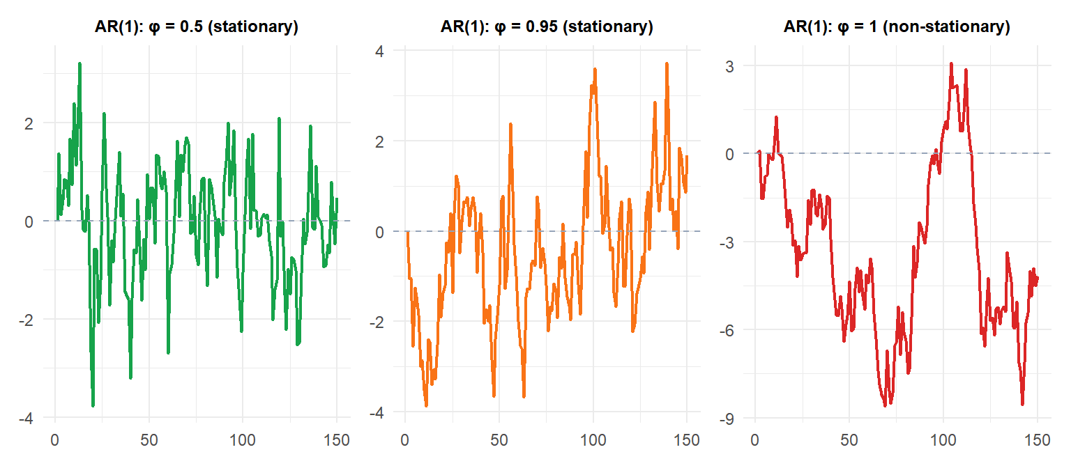
With \(\phi = 0.5\) (green), the series reverts quickly to zero. With \(\phi = 0.95\) (orange), reversion is slow and the series has long memory. With \(\phi = 1\) (red), the random walk drifts without bound.

ACF and PACF of AR processes

The theoretical ACF of a stationary AR(\(p\)) satisfies the Yule-Walker equations:

\[\rho_k = \phi_1 \rho_{k-1} + \phi_2 \rho_{k-2} + \cdots + \phi_p \rho_{k-p}, \quad k \geq 1\]

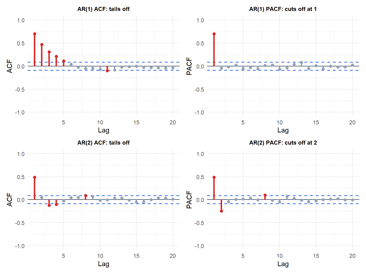
This gives an ACF that tails off geometrically (or with damped oscillations if the roots are complex). The PACF cuts off sharply after lag \(p\): \(\phi_{kk} = 0\) for \(k > p\).

This cut-off in the PACF is the key identifier of AR(\(p\)) models.

Estimation

Ordinary Least Squares (OLS)

Write the AR(\(p\)) as a regression: \(y_t = \phi_1 y_{t-1} + \cdots + \phi_p y_{t-p} + \varepsilon_t\). OLS minimizes \(\sum_{t=p+1}^T \varepsilon_t^2\) and gives consistent, asymptotically efficient estimates when the process is stationary.

Yule-Walker equations

Express the ACF in terms of the parameters using the Yule-Walker equations in matrix form:

\[\begin{pmatrix}\rho_1 \\ \rho_2 \\ \vdots \\ \rho_p\end{pmatrix} = \begin{pmatrix}1 & \rho_1 & \cdots & \rho_{p-1} \\ \rho_1 & 1 & \cdots & \rho_{p-2} \\ \vdots & & \ddots & \vdots \\ \rho_{p-1} & \rho_{p-2} & \cdots & 1\end{pmatrix} \begin{pmatrix}\phi_1 \\ \phi_2 \\ \vdots \\ \phi_p\end{pmatrix}\]

Plugging in the sample ACF \(\hat{\rho}_k\) gives the Yule-Walker estimates. They are less efficient than MLE but guaranteed to produce stationary estimates (all roots outside the unit circle).

Maximum Likelihood Estimation (MLE)

Assumes Gaussian errors and maximizes the joint likelihood. More efficient than OLS or Yule-Walker for small samples. Used by arima() in R by default.

Example: daily temperature AR(1)

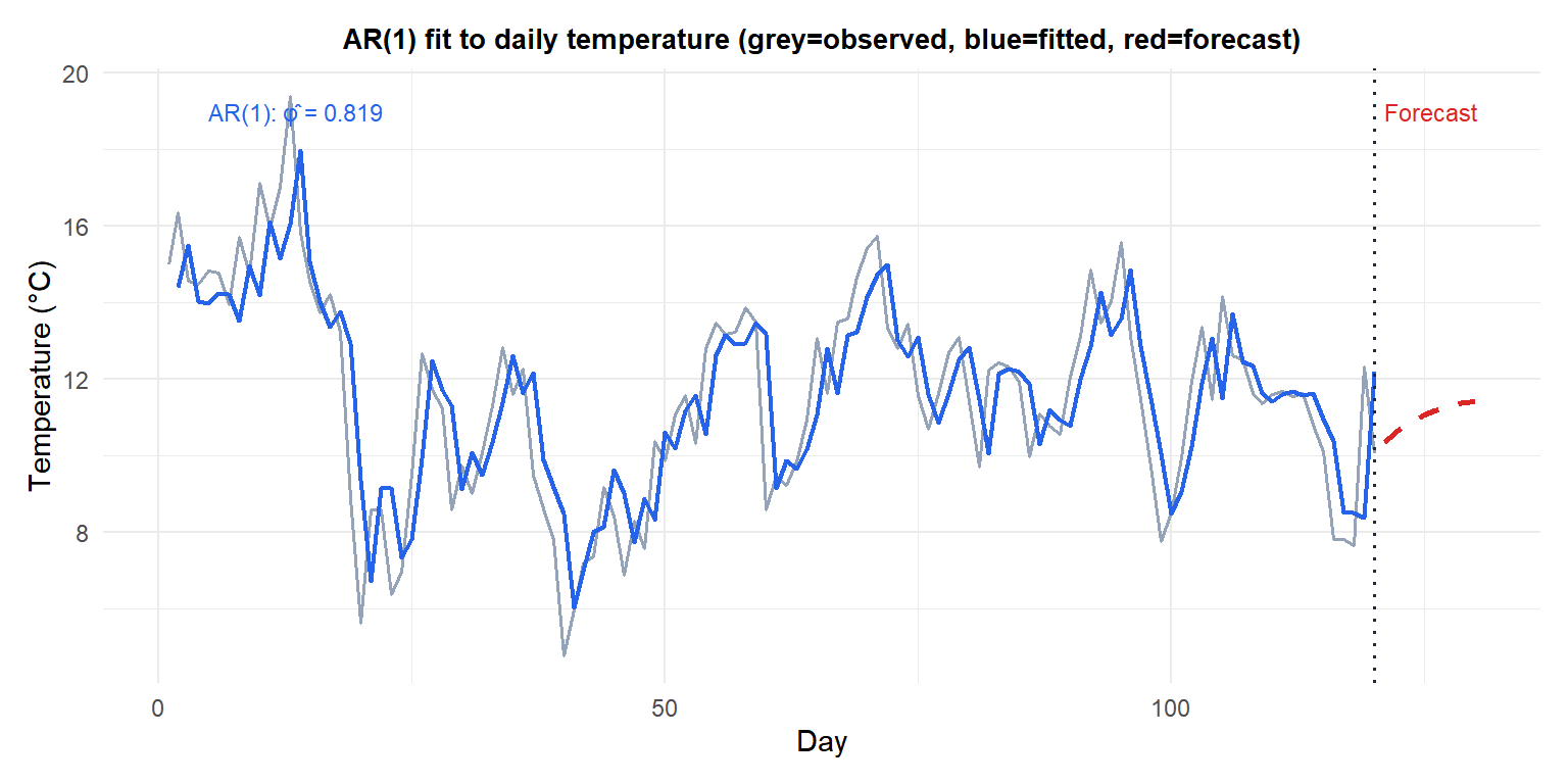
The AR(1) forecast (red) reverts toward the unconditional mean \(\mu = \phi_0/(1-\phi_1)\) as the horizon increases. Multi-step forecasts of AR processes are increasingly uncertain and converge to the long-run mean for \(h \to \infty\).

Order selection

The PACF cuts off at the true order \(p\), providing an initial estimate. Formal selection uses information criteria:

\[\text{AIC} = -2\log\hat{L} + 2(p+1), \qquad \text{BIC} = -2\log\hat{L} + \log(T)(p+1)\]

BIC penalizes complexity more heavily and tends to select smaller models. Both should be compared across a range of candidate orders.

# Fit AR(1) by MLE
arima(y, order = c(1, 0, 0))

# Automatic order selection by AIC
ar(y, method = "mle")

# With AIC/BIC comparison across orders
library(forecast)
auto.arima(y, max.p = 5, max.q = 0, d = 0)  # AR only

# Yule-Walker estimation
ar(y, method = "yule-walker")