Cluster sampling
Cluster sampling selects groups (clusters) rather than individual units. It is the practical choice when no complete sampling frame exists or when geographic dispersion makes individual sampling prohibitively expensive. The cost is lower statistical efficiency: clustered samples contain less information per unit than SRS because units within the same cluster tend to be similar.
When cluster sampling is necessary
Cluster sampling is used when:
- No complete list of population units exists, but a list of natural groups (schools, hospitals, villages, companies) is available.
- The population is geographically dispersed and visiting individual units is too costly.
- Administrative convenience requires working with groups rather than individuals.
Examples: national health surveys (sample districts, then households), educational research (sample schools, then students), market research (sample zip codes, then households).
One-stage vs two-stage cluster sampling
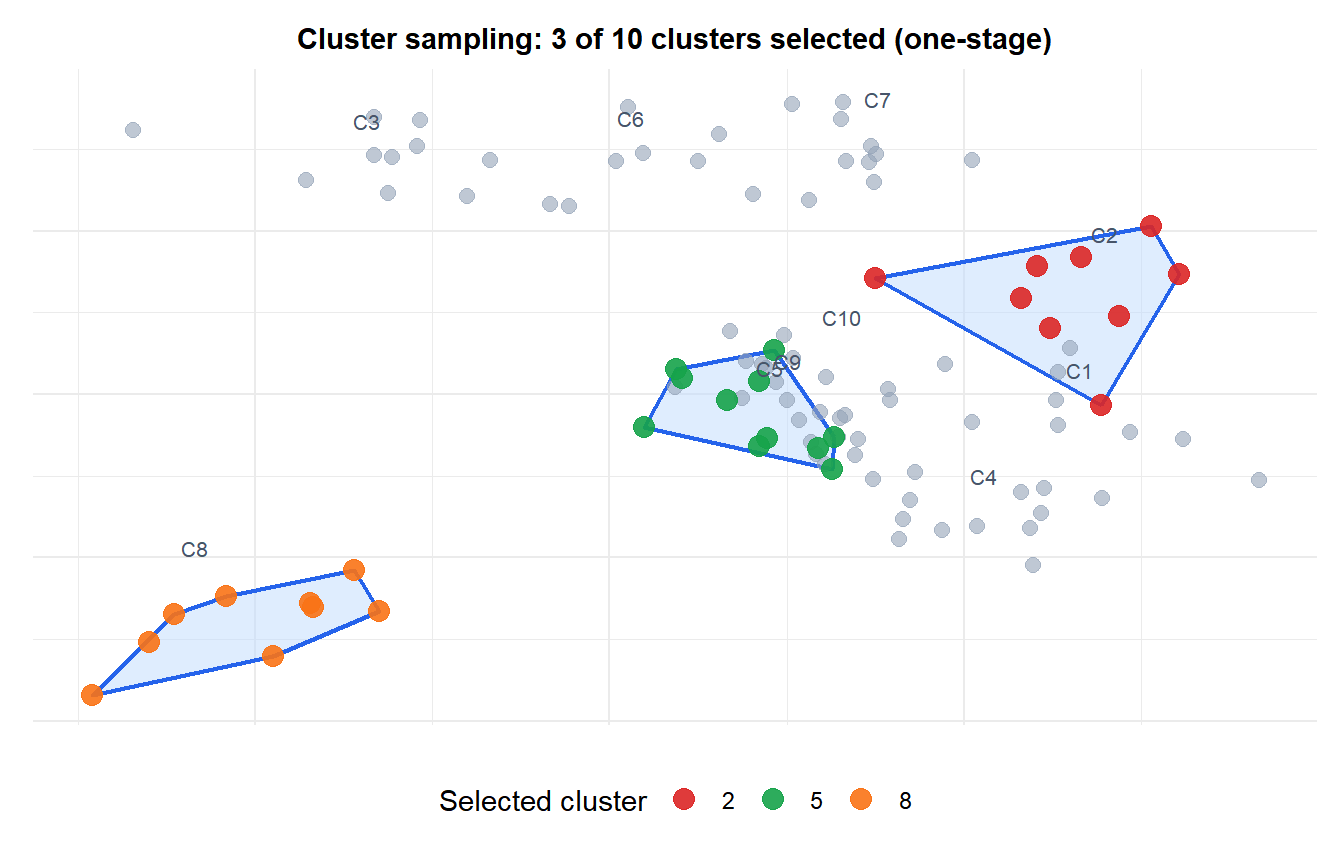
One-stage cluster sampling
Select \(m\) clusters from the \(M\) available clusters. Measure all units within the selected clusters. Simple but can result in large samples if clusters are large.
Two-stage cluster sampling
Select \(m\) clusters (first stage), then draw a random sample of units within each selected cluster (second stage). More flexible: the within-cluster sample size can be controlled independently of the cluster size.
Intraclass correlation and design effect
The key quantity in cluster sampling is the intraclass correlation coefficient (ICC), \(\rho\):
\[\rho = \frac{\text{variance between cluster means}}{\text{total variance}}\]
\(\rho\) measures how similar units within the same cluster are. It ranges from 0 (clusters are no more homogeneous than the population) to 1 (all units within a cluster are identical).
The design effect (DEFF) measures the efficiency loss of cluster sampling relative to SRS of the same total size \(n\):
\[\text{DEFF} = 1 + (m_0 - 1)\rho\]
where \(m_0\) is the average number of units sampled per cluster. The effective sample size is \(n_\text{eff} = n / \text{DEFF}\).
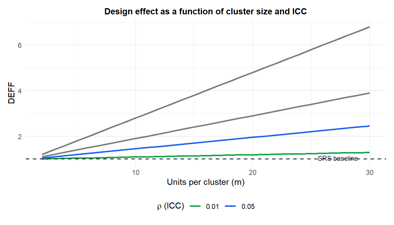
Even a small ICC of 0.05 with 20 units per cluster gives DEFF = \(1 + 19 \times 0.05 = 1.95\): you need nearly twice as many observations to achieve the same precision as SRS.
⚠️ Never treat clustered observations as independent
The most common and serious mistake in cluster sampling analysis: treating the \(n\) individual units as if they were \(n\) independent SRS observations. This underestimates standard errors, narrows confidence intervals, and inflates test statistics, producing spuriously significant results.
Any analysis of cluster-sampled data must account for the clustering, either by:
- Using survey-weighted standard errors (e.g.,
surveypackage in R withsvycluster()). - Including cluster-level random effects in a mixed model.
- Using the design effect to inflate standard errors: \(\text{SE}_\text{adjusted} = \text{SE}_\text{naive} \times \sqrt{\text{DEFF}}\).
This issue affects published research in medicine, education, and social science whenever cluster-randomized trials or multi-site studies are analyzed incorrectly.
Example: national health survey
A ministry of health wants to estimate the proportion of adults with hypertension in a country of 5 million adults. No individual registry exists, but a list of 2,000 primary care centers is available.
Design (two-stage):
- Randomly select 50 centers (clusters) from 2,000.
- Within each selected center, randomly sample 30 patients.
Total sample: \(n = 50 \times 30 = 1{,}500\) patients.
Suppose the ICC for hypertension within centers is \(\rho = 0.08\).
\[\text{DEFF} = 1 + (30 - 1) \times 0.08 = 1 + 2.32 = 3.32\]
\[n_\text{eff} = \frac{1500}{3.32} \approx 452\]
The 1,500 clustered observations provide the same precision as only 452 SRS observations. To match an SRS of 1,500, the clustered design would need \(1500 \times 3.32 \approx 4{,}980\) observations.
For a fixed total cost, reducing cluster size \(m_0\) and increasing the number of clusters \(m\) almost always improves precision. This is because:
- More clusters means more independent pieces of information.
- Fewer units per cluster reduces the redundancy from clustering.
If sampling one cluster costs \(c_1\) (travel, setup) and sampling one unit costs \(c_2\) (interview), the optimal cluster size is:
\[m_\text{opt} = \sqrt{\frac{c_1}{c_2} \cdot \frac{1-\rho}{\rho}}\]
If \(c_1 = 200\), \(c_2 = 10\), \(\rho = 0.05\): \(m_\text{opt} = \sqrt{20 \times 19} \approx 19\) units per cluster. Sampling more than 19 per cluster wastes budget on redundant information.
💡 Cluster vs stratified sampling: the key distinction
Both methods involve groups, but they work oppositely:
- Stratified: all strata are represented; the gain is from within-stratum homogeneity.
- Cluster: only some clusters are selected; the loss is from within-cluster homogeneity (ICC > 0).
Stratified sampling is chosen to increase efficiency. Cluster sampling is chosen for practical necessity (cost, no frame) and almost always reduces efficiency. When both are used together (select clusters, then stratify within clusters), the design is called stratified cluster sampling or multistage sampling.

