Probability mass function
The probability mass function (PMF) assigns a probability to each possible value of a discrete random variable. Unlike the PDF for continuous variables, the PMF gives probabilities directly, not densities: you can read the probability of any outcome straight from the function.
Definition
The probability mass function of a discrete random variable \(X\) is a function \(p(x)\) that gives the probability of each possible outcome:
\[ p(x) = P(X = x) \]
A function \(p(x)\) is a valid PMF if and only if:
- \(p(x) \geq 0\) for all \(x\).
- \(\sum_{x} p(x) = 1\) (probabilities sum to 1 across all possible values).
⚠️ PMF vs PDF: a fundamental difference
With a PMF, you read probabilities directly: (p(3) = P(X = 3)) is a probability. With a PDF, (f(3)) is a density, not a probability, and can exceed 1. Probabilities from a PDF require integration over an interval. Never sum a PDF or integrate a PMF: the tool must match the type of variable.
Common PMFs
Binomial distribution
Models the number of successes in \(n\) independent trials, each with probability \(p\) of success:
\[p(x) = \binom{n}{x} p^x (1-p)^{n-x} \quad \text{for } x = 0, 1, \ldots, n\]
A factory produces items where each has a 20% defect rate. A batch of 10 items is inspected. Let (X) = number of defective items, (X \sim \text{Binomial}(10, 0.2)).
- \(P(X = 0) = \binom{10}{0}(0.2)^0(0.8)^{10} \approx 0.107\): about 11% of batches are defect-free.
- \(P(X = 2) = \binom{10}{2}(0.2)^2(0.8)^8 \approx 0.302\): the most likely outcome.
- \(P(X \geq 4) = 1 - P(X \leq 3) \approx 1 - 0.879 = 0.121\): about 12% of batches have 4 or more defects.

Poisson distribution
Models the number of events occurring in a fixed interval of time or space, when events happen at a constant average rate \(\lambda\) and independently of each other:
\[p(x) = \frac{\lambda^x e^{-\lambda}}{x!} \quad \text{for } x = 0, 1, 2, \ldots\]
A bank branch receives an average of 3 customers per minute during peak hours. Let (X) = number of customers in one minute, (X \sim \text{Poisson}(3)).
- \(P(X = 0) = \frac{3^0 e^{-3}}{0!} = e^{-3} \approx 0.050\): 5% chance of no arrivals in a minute.
- \(P(X = 3) = \frac{3^3 e^{-3}}{3!} = \frac{27 e^{-3}}{6} \approx 0.224\): most likely outcome.
- \(P(X > 5) = 1 - P(X \leq 5) \approx 1 - 0.916 = 0.084\): about 8% chance of 6 or more arrivals.
Geometric distribution
Models the number of trials needed to get the first success, where each trial has probability \(p\) of success:
\[p(x) = (1-p)^{x-1} p \quad \text{for } x = 1, 2, 3, \ldots\]
A salesperson closes a deal with probability 0.3 on each call, independently. Let (X) = number of calls until the first sale.
- \(P(X = 1) = 0.3\): 30% chance of closing on the first call.
- \(P(X = 3) = (0.7)^2 \times 0.3 = 0.147\): about 15% chance of needing exactly 3 calls.
- \(P(X > 5) = (0.7)^5 \approx 0.168\): about 17% chance of needing more than 5 calls.
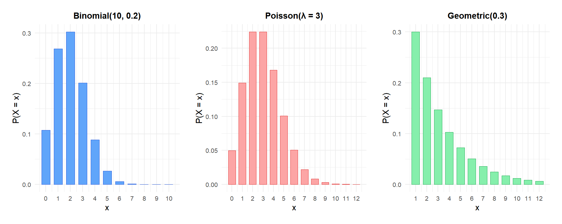
Figure 1: PMF of three common discrete distributions: Binomial(10, 0.2), Poisson(3), and Geometric(0.3)
Relationship with the CDF
The CDF of a discrete random variable is obtained by summing the PMF:
\[F(x) = P(X \leq x) = \sum_{t \leq x} p(t)\]
Conversely, for any two consecutive values \(x_{i}\) and \(x_{i+1}\):
\[p(x_i) = F(x_i) - F(x_{i-1})\]
You can recover the PMF from the CDF by taking differences, just as you recover the PDF from the CDF by differentiation.
💡 Choosing the right discrete distribution
- Fixed number of trials, each success/failure: Binomial.
- Number of events in a fixed time or space interval, at a constant average rate: Poisson.
- Number of trials until the first success: Geometric.
- Number of trials until the \(k\)-th success: Negative Binomial.
- Sampling without replacement from a finite population: Hypergeometric.

