Independent events
Two events are independent when knowing that one occurred gives no information about whether the other occurred. Independence is a property of the probabilistic model, not just of the physical setup, and it must be verified rather than assumed.
Definition
Events \(A\) and \(B\) are independent if and only if:
\[P(A \cap B) = P(A) \times P(B)\]
An equivalent condition: \(A\) and \(B\) are independent if and only if \(P(A \mid B) = P(A)\), that is, knowing \(B\) occurred does not change the probability of \(A\). Both formulations say the same thing.
For \(n\) events \(A_1, A_2, \ldots, A_n\) to be mutually independent, the product rule must hold for every subset:
\[P(A_i \cap A_j) = P(A_i)P(A_j) \quad \text{for all } i \neq j\] \[P(A_i \cap A_j \cap A_k) = P(A_i)P(A_j)P(A_k) \quad \text{for all } i < j < k\] \[\vdots\] \[P(A_1 \cap \cdots \cap A_n) = P(A_1) \cdots P(A_n)\]
All \(2^n - n - 1\) conditions must hold simultaneously.
How to verify independence
The formal test is straightforward: compute \(P(A \cap B)\), \(P(A)\), and \(P(B)\), then check whether \(P(A \cap B) = P(A) \times P(B)\).
An analysis of 1,000 email subscribers finds:
| Clicked link | Did not click | Total | |
|---|---|---|---|
| Opened email | 180 | 220 | 400 |
| Did not open | 120 | 480 | 600 |
| Total | 300 | 700 | 1,000 |
Let \(O\) = opened, \(C\) = clicked.
\[P(O) = 400/1000 = 0.40, \quad P(C) = 300/1000 = 0.30\] \[P(O \cap C) = 180/1000 = 0.18\]
Test: \(P(O) \times P(C) = 0.40 \times 0.30 = 0.12 \neq 0.18\)
The events are not independent: subscribers who opened the email are much more likely to click than those who did not. \(P(C \mid O) = 180/400 = 0.45 \neq 0.30 = P(C)\).
A factory has two machines on separate lines with no shared components. Machine A fails with probability 0.04, machine B with probability 0.03. In 10,000 production days, both failed on 12 days.
\[P(A \cap B) = 12/10000 = 0.0012\] \[P(A) \times P(B) = 0.04 \times 0.03 = 0.0012 \checkmark\]
The failures are independent: consistent with the machines having no shared components or common causes.
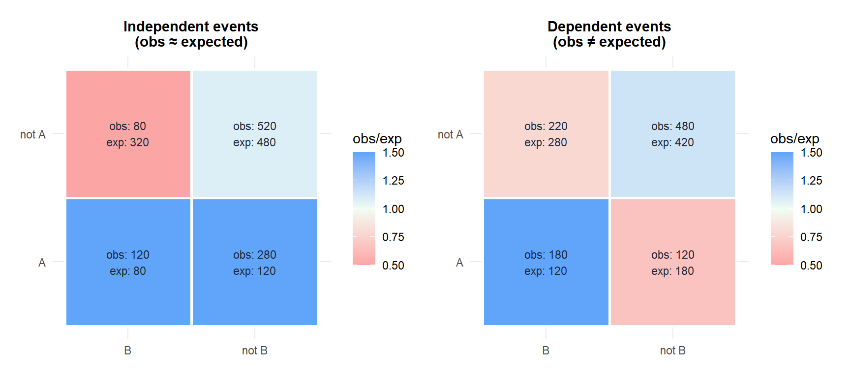
In the left panel (independent), observed and expected frequencies match: all cells are near white (ratio \(\approx 1\)). In the right panel (dependent), the top-left cell (both \(A\) and \(B\)) is blue (observed > expected) while the bottom-left (not \(A\), but \(B\)) is red (observed < expected), revealing the dependence structure.
Common misconceptions
Independence vs mutual exclusivity
⚠️ Mutually exclusive events with positive probability are never independent
If \(A\) and \(B\) are mutually exclusive (\(A \cap B = \emptyset\)), then \(P(A \cap B) = 0\). For independence we would need \(P(A) \times P(B) = 0\), which requires at least one of them to have probability zero.
Intuitively: if \(A\) and \(B\) cannot both happen, then knowing \(A\) occurred tells you immediately that \(B\) did not. That is the opposite of independence.
Example: in a single server request, the events “response time under 100 ms” and “response time over 500 ms” are mutually exclusive. If you know the response was fast, you know it was not slow. They are maximally dependent, not independent.
Independence vs zero correlation
⚠️ Zero correlation does not imply independence
Two random variables (or events) can be uncorrelated but still dependent. The classic example: let \(X \sim \text{Uniform}(-1, 1)\) and \(Y = X^2\). Then \(\text{Cov}(X, Y) = 0\) (zero correlation), but \(Y\) is completely determined by \(X\): they are maximally dependent.
For events specifically: two events can have \(P(A \cap B) \neq P(A) \times P(B)\) even when their “correlation” in the colloquial sense appears low. Always use the formal independence test, not intuition about correlation.
Pairwise vs mutual independence
Three events can be independent in pairs but not mutually independent. A classic example (Bernstein):
Consider two fair coin flips. Define:
- \(A\) = first flip is heads.
- \(B\) = second flip is heads.
- \(C\) = exactly one flip is heads.
Then \(P(A) = P(B) = P(C) = 0.5\), and:
- \(P(A \cap B) = 0.25 = P(A)P(B)\) ✓
- \(P(A \cap C) = 0.25 = P(A)P(C)\) ✓
- \(P(B \cap C) = 0.25 = P(B)P(C)\) ✓
But \(P(A \cap B \cap C) = 0 \neq 0.5^3 = 0.125\). The three events are pairwise independent but not mutually independent.
Real-world examples
System reliability
A critical system has three independent backup servers. Each server is available with probability 0.95. The system works if at least one server is available.
\[P(\text{all fail}) = (1 - 0.95)^3 = 0.05^3 = 0.000125\]
\[P(\text{system works}) = 1 - 0.000125 = 0.999875\]
Independence here is justified by the servers being physically separate with no shared power supply or network components.
Clinical trial with two endpoints
A drug trial measures two outcomes: reduction in blood pressure (\(A\)) and reduction in cholesterol (\(B\)). After analysis:
\[P(A) = 0.60, \quad P(B) = 0.45, \quad P(A \cap B) = 0.27\]
Test: \(P(A) \times P(B) = 0.60 \times 0.45 = 0.27 = P(A \cap B)\)
The two outcomes are independent in this trial: whether a patient responds on blood pressure gives no information about their cholesterol response. This finding has implications for the drug’s mechanism of action.
Password security
A password must pass three independent security checks: length (\(L\)), special characters (\(C\)), and not appearing in a known list (\(N\)). Each check passes with probability 0.8 independently.
\[P(\text{all checks pass}) = 0.8^3 = 0.512\]
\[P(\text{at least one fails}) = 1 - 0.512 = 0.488\]
Nearly half of all passwords fail at least one check.
💡 When is independence a reasonable assumption?
Independence is a modelling choice. It is reasonable when:
- Events arise from physically separate processes with no shared components or causes.
- Observations are drawn randomly from a large population (sampling with replacement, or without replacement from a very large population).
- Trials are repeated under identical, non-interacting conditions.
It is not reasonable when events share a common cause (two machines from the same batch), when outcomes influence each other (disease spreading between people in contact), or when sampling without replacement from a small population.

