Conditional probability
Conditional probability answers the question: given that we know \(B\) occurred, how does that change the probability of \(A\)? It is the foundation of Bayesian reasoning, medical testing, spam filters, and any situation where new information updates our uncertainty.
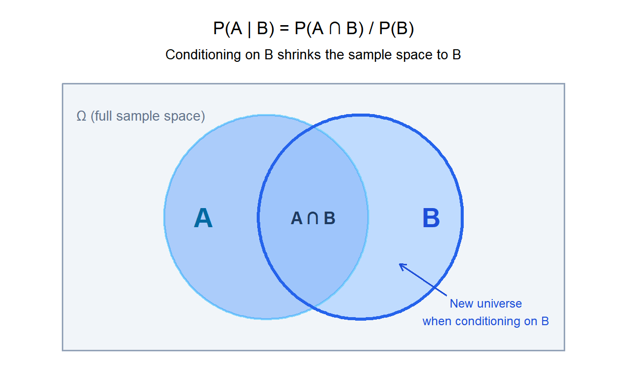
Definition
The conditional probability of \(A\) given \(B\) is the probability that \(A\) occurs, restricted to the cases where \(B\) has already occurred:
\[P(A \mid B) = \frac{P(A \cap B)}{P(B)}, \quad P(B) > 0\]
Geometrically, conditioning on \(B\) means we shrink the sample space to \(B\) and ask what fraction of \(B\) is also in \(A\). The formula divides the overlap \(P(A \cap B)\) by the new “universe” \(P(B)\).
From this definition, the multiplication rule follows immediately:
\[P(A \cap B) = P(A \mid B) \cdot P(B) = P(B \mid A) \cdot P(A)\]
⚠️ P(A|B) ≠ P(B|A): the most important asymmetry in probability
\(P(A \mid B)\) and \(P(B \mid A)\) are completely different quantities. Confusing them has serious consequences:
- \(P(\text{positive test} \mid \text{has disease})\) is the test sensitivity - what the lab reports.
- \(P(\text{has disease} \mid \text{positive test})\) is what the patient wants to know - and it depends critically on how rare the disease is.
In the legal context this is called the prosecutor’s fallacy: confusing \(P(\text{evidence} \mid \text{innocent})\) with \(P(\text{innocent} \mid \text{evidence})\). Several wrongful convictions have been linked to this error.
Law of total probability
To compute \(P(B)\) in the denominator of the conditional probability formula, we often need to account for all the ways \(B\) can happen. If \(A_1, A_2, \ldots, A_n\) form a partition of the sample space (mutually exclusive and exhaustive), then:
\[P(B) = \sum_{i=1}^{n} P(B \mid A_i) \cdot P(A_i)\]
This is the law of total probability. It decomposes \(P(B)\) into contributions from each scenario \(A_i\).
A factory has three production lines contributing 50%, 30%, and 20% of output. Their defect rates are 2%, 4%, and 6% respectively. What is the overall defect rate?
\[P(\text{defect}) = 0.02 \times 0.50 + 0.04 \times 0.30 + 0.06 \times 0.20\] \[= 0.010 + 0.012 + 0.012 = 0.034\]
The overall defect rate is 3.4%.
Step-by-step examples
Example 1: medical test (complete calculation)
A disease affects 1% of the population (\(P(D) = 0.01\)). A diagnostic test has: - Sensitivity: \(P(\text{pos} \mid D) = 0.95\) (detects 95% of true cases). - False positive rate: \(P(\text{pos} \mid D^c) = 0.05\) (flags 5% of healthy people).
A patient tests positive. What is the probability they have the disease?
Step 1: compute \(P(\text{pos})\) using the law of total probability:
\[P(\text{pos}) = P(\text{pos} \mid D) \cdot P(D) + P(\text{pos} \mid D^c) \cdot P(D^c)\] \[= 0.95 \times 0.01 + 0.05 \times 0.99 = 0.0095 + 0.0495 = 0.059\]
Step 2: apply the conditional probability formula:
\[P(D \mid \text{pos}) = \frac{P(\text{pos} \mid D) \cdot P(D)}{P(\text{pos})} = \frac{0.0095}{0.059} \approx 0.161\]
Only 16% of people who test positive actually have the disease. The test is accurate, but the disease is rare enough that most positive results are false alarms. This is the base rate effect: the prior probability of having the disease (\(P(D) = 0.01\)) dominates.
Instead of probabilities, think about 10,000 people:
- 100 have the disease. Of those, \(95\) test positive (true positives).
- 9,900 are healthy. Of those, \(495\) test positive (false positives).
Total positives: \(95 + 495 = 590\).
\(P(D \mid \text{pos}) = 95/590 \approx 0.161\). Same answer, much more intuitive.
This frequency approach (natural frequencies) is recommended by statisticians when communicating risk to patients or policymakers.
Example 2: sequential hiring process
A company’s hiring process has two stages. Historical data shows: - 40% of applicants pass the first interview: \(P(S_1) = 0.40\). - Of those, 35% pass the second interview: \(P(S_2 \mid S_1) = 0.35\).
Probability of passing both:
\[P(S_1 \cap S_2) = P(S_2 \mid S_1) \cdot P(S_1) = 0.35 \times 0.40 = 0.14\]
14% of applicants make it through both rounds.
Now suppose we know a candidate passed the second interview. What is the probability they also passed the first? (They must have, since stage 2 requires stage 1.)
\[P(S_1 \mid S_2) = \frac{P(S_1 \cap S_2)}{P(S_2)}\]
We need \(P(S_2)\). Since you cannot reach stage 2 without passing stage 1: \(P(S_2) = P(S_1 \cap S_2) = 0.14\).
\[P(S_1 \mid S_2) = \frac{0.14}{0.14} = 1\]
As expected: if you passed stage 2, you necessarily passed stage 1.
Example 3: spam filter
A spam filter analyzes the word “free” in emails: - 60% of spam emails contain “free”: \(P(\text{free} \mid \text{spam}) = 0.60\). - 5% of legitimate emails contain “free”: \(P(\text{free} \mid \text{legit}) = 0.05\). - 30% of incoming emails are spam: \(P(\text{spam}) = 0.30\).
An email containing “free” arrives. What is the probability it is spam?
\[P(\text{free}) = 0.60 \times 0.30 + 0.05 \times 0.70 = 0.180 + 0.035 = 0.215\]
\[P(\text{spam} \mid \text{free}) = \frac{0.60 \times 0.30}{0.215} = \frac{0.18}{0.215} \approx 0.837\]
84% probability of spam given the word “free”. Real spam filters apply this logic to hundreds of words simultaneously using Naive Bayes classification.
Connection to independence
Events \(A\) and \(B\) are independent if and only if:
\[P(A \mid B) = P(A)\]
That is, knowing \(B\) occurred does not change the probability of \(A\). When this holds, the conditional probability formula gives \(P(A \cap B) = P(A) \cdot P(B)\), which is the definition of independence.
Conditional probability is therefore the general case: independence is the special case where conditioning has no effect.
💡 Conditional probability changes the sample space
The key intuition: conditioning on \(B\) replaces the original sample space \(\Omega\) with the restricted space \(B\). All probabilities are then re-computed within this smaller universe. This is why \(P(A \mid B)\) can be very different from \(P(A)\): we are asking a completely different question. Not “how often does \(A\) happen?” but “among the cases where \(B\) happened, how often does \(A\) also happen?”

