Simplex method
The Simplex method, developed by George Dantzig in 1947, solves linear programs by exploiting the fact that the optimal solution always lies at a vertex of the feasible polytope. It moves from vertex to vertex along edges, always improving the objective function, until no improving neighbor exists.
Key idea
A linear program with \(n\) variables and \(m\) constraints (in standard form, after adding \(m\) slack variables) has at most \(\binom{n+m}{m}\) vertices. The Simplex method never evaluates all of them: it starts at one vertex and moves to an adjacent better vertex at each iteration. In practice it terminates in \(O(m)\) to \(O(2m)\) pivots for most real problems.
Each vertex corresponds to a basic feasible solution (BFS): a solution where exactly \(m\) variables are nonzero (the basic variables) and the remaining \(n\) are zero (the nonbasic variables). The idea of restricting attention to vertices reduces an infinite search space to a finite one.
Standard form and the initial tableau
Any LP with inequality constraints is first converted to standard form by adding slack variables. For a maximization problem \(\max z = \mathbf{c}^T x\) subject to \(\mathbf{A}x \leq \mathbf{b}\), \(x \geq 0\):
\[\mathbf{A}x + s = \mathbf{b}, \qquad x \geq 0,\; s \geq 0\]
The slack variables \(s_i\) absorb the slack in each inequality. The initial BFS is \(x = 0\), \(s = \mathbf{b}\), \(z = 0\): start at the origin with all slacks in the basis.
The Simplex tableau organizes the system:
\[\begin{array}{c|ccccc|c} \text{Basis} & x_1 & x_2 & \cdots & s_1 & s_2 & \text{RHS} \\\hline s_1 & a_{11} & a_{12} & \cdots & 1 & 0 & b_1 \\ s_2 & a_{21} & a_{22} & \cdots & 0 & 1 & b_2 \\\hline -z & -c_1 & -c_2 & \cdots & 0 & 0 & 0 \end{array}\]
The objective row stores \(-\mathbf{c}^T\) (negative because we write \(-z + \mathbf{c}^T x = 0\) and track improvements as we drive \(-z\) toward its most negative value, i.e., maximize \(z\)).
The algorithm: three rules
Rule 1: entering variable (most negative coefficient)
Scan the objective row. The nonbasic variable with the most negative coefficient enters the basis: bringing it from zero to a positive value will increase \(z\) the fastest. If all coefficients are \(\geq 0\), the current BFS is optimal.
Rule 2: leaving variable (minimum ratio test)
For the entering column, compute the ratio \(b_i / a_{i,\text{enter}}\) for every row \(i\) where \(a_{i,\text{enter}} > 0\). The basic variable in the row with the smallest ratio leaves the basis. This ratio is how much the entering variable can increase before the current basic variable in that row hits zero (its lower bound). Taking the minimum ensures we stay feasible.
If no ratio is positive (all \(a_{i,\text{enter}} \leq 0\)), the LP is unbounded: the entering variable can grow without limit.
Rule 3: pivot operation
The element at the intersection of the entering column and leaving row is the pivot element. Divide the pivot row by the pivot element to make the pivot equal to 1. Then use row operations to eliminate the entering variable from every other row, including the objective row. Update the basis label.
Repeat until the optimality condition is met.
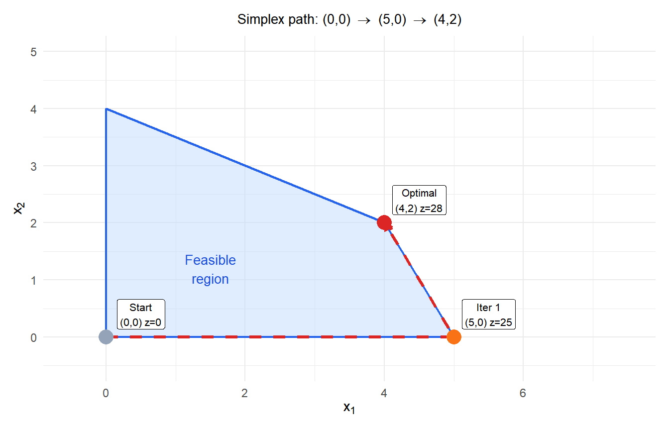
Complete example: two iterations
Maximize \(z = 5x_1 + 4x_2\) subject to:
\[x_1 + 2x_2 \leq 8, \qquad 2x_1 + x_2 \leq 10, \qquad x_1, x_2 \geq 0\]
Initial tableau (BFS: \(x_1=x_2=0\), \(s_1=8\), \(s_2=10\), \(z=0\)):
\[\begin{array}{c|cccc|c} \text{Basis} & x_1 & x_2 & s_1 & s_2 & \text{RHS} \\\hline s_1 & 1 & 2 & 1 & 0 & 8 \\ s_2 & \mathbf{2} & 1 & 0 & 1 & 10 \\\hline -z & -5 & -4 & 0 & 0 & 0 \end{array}\]
Iteration 1:
Entering: \(x_1\) (most negative: \(-5\)). Ratios: \(8/1 = 8\), \(10/2 = 5\). Minimum is 5, so \(s_2\) leaves. Pivot element: 2 (row 2, column \(x_1\)).
Divide row 2 by 2. Eliminate \(x_1\) from row 1 (subtract \(1 \times\) new row 2) and from objective row (add \(5 \times\) new row 2):
\[\begin{array}{c|cccc|c} \text{Basis} & x_1 & x_2 & s_1 & s_2 & \text{RHS} \\\hline s_1 & 0 & \mathbf{1.5} & 1 & -0.5 & 3 \\ x_1 & 1 & 0.5 & 0 & 0.5 & 5 \\\hline -z & 0 & -1.5 & 0 & 2.5 & 25 \end{array}\]
BFS: \(x_1=5\), \(x_2=0\), \(s_1=3\), \(z=25\). Objective coefficient \(-1.5 < 0\): not yet optimal.
Iteration 2:
Entering: \(x_2\) (only negative: \(-1.5\)). Ratios: \(3/1.5 = 2\), \(5/0.5 = 10\). Minimum is 2, so \(s_1\) leaves. Pivot element: 1.5.
Divide row 1 by 1.5. Eliminate \(x_2\) from row 2 and from objective row:
\[\begin{array}{c|cccc|c} \text{Basis} & x_1 & x_2 & s_1 & s_2 & \text{RHS} \\\hline x_2 & 0 & 1 & 2/3 & -1/3 & 2 \\ x_1 & 1 & 0 & -1/3 & 2/3 & 4 \\\hline -z & 0 & 0 & 1 & 2 & 28 \end{array}\]
All objective coefficients \(\geq 0\). Optimal solution: \(x_1 = 4\), \(x_2 = 2\), \(z = 28\).
Finding an initial BFS: the Big M method
The origin (\(x = 0\), \(s = \mathbf{b}\)) is a valid initial BFS only when all \(b_i \geq 0\). If some constraints are \(\geq\) or \(=\) type, slack variables alone do not give a BFS. The Big M method adds artificial variables \(a_i \geq 0\) to these rows and penalizes them heavily in the objective:
\[\max z = \mathbf{c}^T x - M \sum_i a_i\]
where \(M\) is a very large number. The initial BFS uses the artificial variables as the basis. If the LP is feasible, Simplex will drive all \(a_i\) to zero. If any \(a_i > 0\) at optimality, the original LP is infeasible.
Maximize \(z = 3x_1 + 2x_2\) subject to \(x_1 + x_2 = 4\), \(x_1, x_2 \geq 0\).
The equality constraint has no slack variable. Add artificial variable \(a_1\):
\[\max z = 3x_1 + 2x_2 - M a_1 \qquad x_1 + x_2 + a_1 = 4, \quad a_1 \geq 0\]
Initial BFS: \(x_1 = x_2 = 0\), \(a_1 = 4\). Simplex will pivot \(a_1\) out and find the optimal \(x_1 = 4\), \(x_2 = 0\), \(z = 12\).
An alternative is the Two-Phase method: Phase I minimizes \(\sum a_i\) to find a feasible BFS (ignoring the original objective); Phase II then optimizes the original objective starting from that BFS.
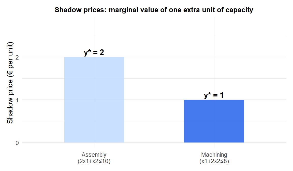
Shadow prices and sensitivity analysis
The final tableau contains more information than just the optimal solution. The objective row coefficients of the slack variables are the shadow prices (dual variables) \(y_i^*\): they measure how much \(z\) increases per unit increase in the RHS \(b_i\).
From the final tableau above: the coefficient of \(s_1\) is 1 and the coefficient of \(s_2\) is 2. So:
- Relaxing constraint 1 (\(x_1 + 2x_2 \leq 8\)) by 1 unit increases optimal \(z\) by €1.
- Relaxing constraint 2 (\(2x_1 + x_2 \leq 10\)) by 1 unit increases optimal \(z\) by €2.
Constraint 2 (assembly) is more valuable: adding one hour of assembly capacity is worth twice as much as adding one hour of machining capacity.
Shadow prices are only valid within a range of \(b_i\) changes (the RHS ranging). Beyond that range, the optimal basis changes and a new Simplex run is needed.
Degeneracy and cycling
A BFS is degenerate if one or more basic variables equal zero. At a degenerate vertex, a pivot may leave the objective value unchanged (a degenerate pivot). In rare cases this causes cycling: the algorithm revisits the same BFS repeatedly without terminating.
Bland’s rule prevents cycling: among all eligible entering variables, choose the one with the smallest index; among all eligible leaving variables, choose the one with the smallest index. This guarantees termination at the cost of possibly slower convergence. In practice, cycling is extremely rare and most implementations use perturbation methods instead.
Simplex vs interior point methods
| Simplex | Interior point (Karmarkar) | |
|---|---|---|
| Path | Along vertices and edges | Through the interior of the feasible region |
| Worst-case complexity | Exponential | Polynomial |
| Practical performance | Very fast (usually \(O(m)\) pivots) | Competitive for very large LPs |
| Warm starting | Easy (reuse basis) | Harder |
| Sensitivity analysis | Direct from final tableau | Requires extra computation |
| Best for | Medium LPs, re-optimization, MIP branch-and-bound | Very large LPs (\(> 10^6\) variables) |
Modern solvers (Gurobi, CPLEX, HiGHS) implement both and switch automatically based on problem size and structure.
⚠️ Simplex can be exponentially slow on adversarial inputs
Klee and Minty (1972) constructed a family of LPs with \(n\) variables where the standard Simplex visits all \(2^n\) vertices. The problem looks like a distorted hypercube. However, such adversarial inputs never arise from real-world applications. For practical problems, Simplex is remarkably fast despite the worst-case guarantee. If you encounter a Simplex run that does not terminate quickly, suspect degeneracy or poor scaling rather than adversarial structure.
💡 Simplex in R
library(lpSolve)

obj <- c(5, 4)
mat <- matrix(c(1, 2, 2, 1), nrow=2, byrow=TRUE)
rhs <- c(8, 10)
dir <- c("<=", "<=")

sol <- lp("max", obj, mat, dir, rhs, compute.sens=TRUE)
sol$solution        # x1=4, x2=2
sol$objval          # 28
sol$duals           # shadow prices: c(1, 2, 0, 0)
sol$sens.coef.from  # lower range for obj coefficients
sol$sens.coef.to    # upper range for obj coefficients
For larger problems, the HiGHS solver (via the highs package) is faster and more robust than lpSolve.

