Linear programming
Linear programming (LP) optimizes a linear objective function over a feasible region defined by linear inequality and equality constraints. It is the foundation of operations research and the problem that the Simplex method solves. The key geometric insight: the optimal solution always lies at a vertex of the feasible polytope.
Standard formulation
A linear program in standard form:
\[\min_{x} \mathbf{c}^T x \quad \text{subject to} \quad \mathbf{A}x = \mathbf{b},\quad x \geq \mathbf{0}\]
where \(x \in \mathbb{R}^n\) are the decision variables, \(\mathbf{c} \in \mathbb{R}^n\) are the objective coefficients, \(\mathbf{A} \in \mathbb{R}^{m \times n}\) is the constraint matrix, and \(\mathbf{b} \in \mathbb{R}^m\) are the right-hand side values.
Any LP with inequality constraints \(\mathbf{A}x \leq \mathbf{b}\) can be converted to standard form by introducing slack variables \(s \geq 0\):
\[\mathbf{A}x + s = \mathbf{b}, \quad x \geq 0, \quad s \geq 0\]
A maximization problem \(\max \mathbf{c}^T x\) is converted by minimizing \(-\mathbf{c}^T x\).
Geometry: why the optimum is at a vertex
The feasible region \(\mathcal{F} = \{x : \mathbf{A}x \leq \mathbf{b},\, x \geq 0\}\) is a convex polytope: the intersection of finitely many half-spaces. Since \(f(x) = \mathbf{c}^T x\) is linear (and therefore convex), its minimum over a convex set is attained at an extreme point, a vertex of the polytope.
This is the key fact that makes LP tractable: instead of searching all of \(\mathcal{F}\) (infinitely many points), we only need to check the vertices (finitely many). The Simplex method exploits this by moving from vertex to vertex along edges, always improving the objective.
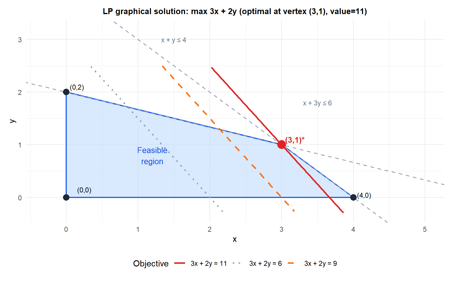
The shaded region is the feasible set. The objective contours (lines of equal value) are pushed in the direction of increasing \(3x+2y\). The optimum is at vertex \((3,1)\) where \(3(3)+2(1)=11\): the last vertex touched before leaving the feasible region.
Complete example: production planning
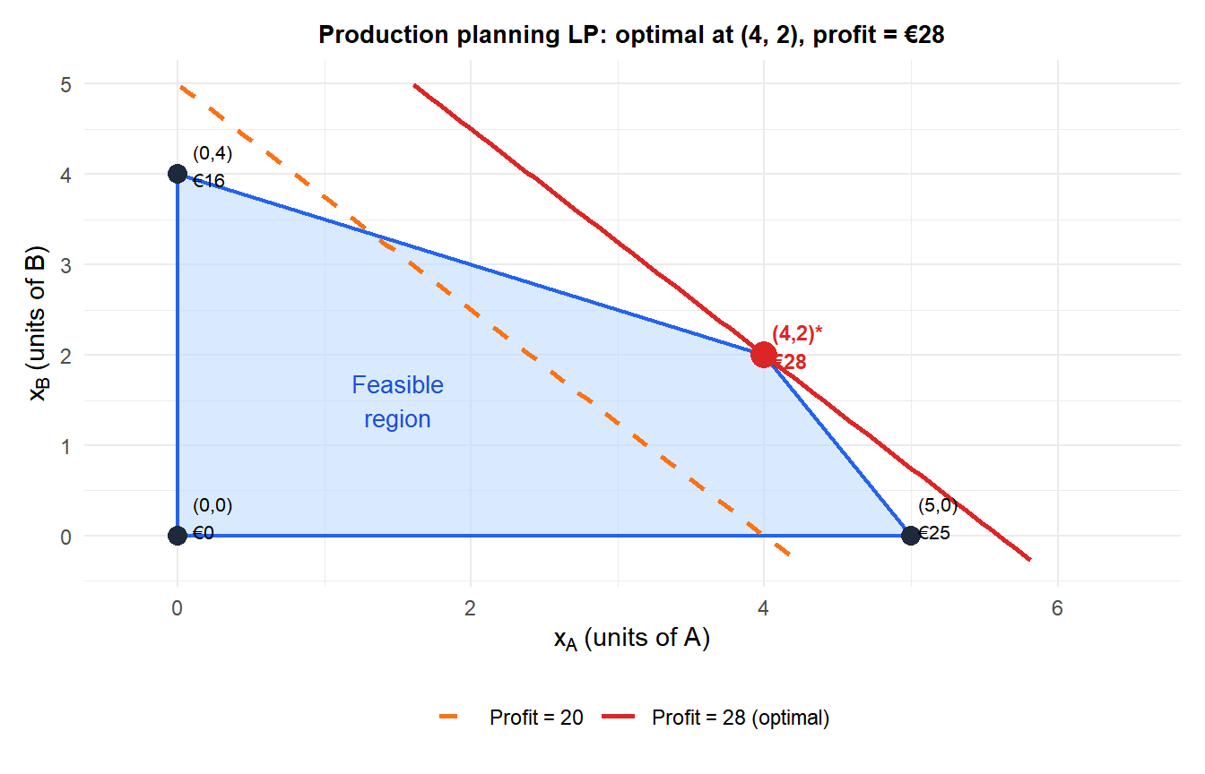
A factory produces two products, A and B. Each unit of A requires 1 hour of machining and 2 hours of assembly. Each unit of B requires 2 hours of machining and 1 hour of assembly. Available: 8 hours machining, 10 hours assembly per day. Profit: €5 per unit of A, €4 per unit of B.
Formulation:
\[\max\; 5x_A + 4x_B\]
\[\text{subject to:} \quad x_A + 2x_B \leq 8 \quad \text{(machining)}\]
\[2x_A + x_B \leq 10 \quad \text{(assembly)}\]
\[x_A, x_B \geq 0\]
Vertices of the feasible region:
| Vertex | \(x_A\) | \(x_B\) | Profit |
|---|---|---|---|
| \((0, 0)\) | 0 | 0 | 0 |
| \((5, 0)\) | 5 | 0 | 25 |
| \((4, 2)\) | 4 | 2 | 28 |
| \((0, 4)\) | 0 | 4 | 16 |
The intersection of the two binding constraints gives \((4, 2)\): solve \(x_A + 2x_B = 8\) and \(2x_A + x_B = 10\) simultaneously.
Optimal solution: produce 4 units of A and 2 units of B for a profit of €28.
Special cases
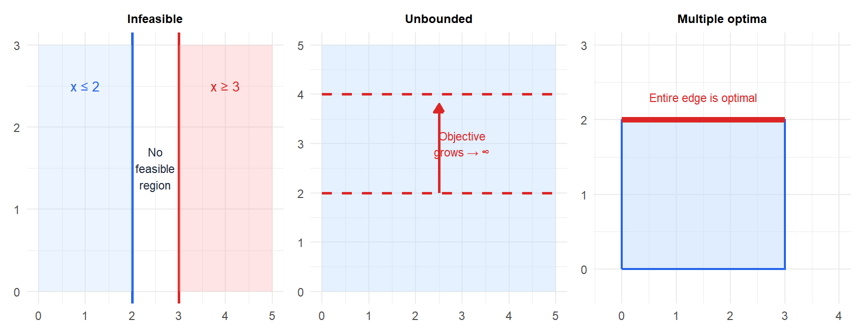
⚠️ Three situations where the LP has no unique finite optimum
1. Infeasible problem: the constraints are contradictory and the feasible region is empty. Example: requiring \(x \geq 5\) and \(x \leq 3\) simultaneously. The LP has no solution.
2. Unbounded problem: the feasible region extends to infinity in the direction of improvement. Example: maximizing \(x\) with only the constraint \(x \geq 0\). The LP has no finite optimum. Always check that your problem is bounded.
3. Multiple optima: the objective function is parallel to one of the constraint boundaries. The optimum is achieved at every point on a face (edge in 2D) of the polytope, not just a single vertex. Any convex combination of the two optimal vertices is also optimal.
Duality
Every LP (the primal) has an associated dual LP. For the primal \(\min \mathbf{c}^T x\) s.t. \(\mathbf{A}x \geq \mathbf{b}\), \(x \geq 0\), the dual is:
\[\max \mathbf{b}^T y \quad \text{s.t.} \quad \mathbf{A}^T y \leq \mathbf{c},\quad y \geq 0\]
Strong duality: if the primal has a finite optimal value, so does the dual, and they are equal: \(\mathbf{c}^T x^* = \mathbf{b}^T y^*\). The dual variables \(y^*\) are the shadow prices: they measure how much the optimal objective improves if the corresponding constraint is relaxed by one unit.
💡 LP in R
library(lpSolve)

# Production planning example: max 5*xA + 4*xB
obj  <- c(5, 4)
mat  <- matrix(c(1,2, 2,1), nrow=2, byrow=TRUE)
rhs  <- c(8, 10)
dir  <- c("<=", "<=")

sol  <- lp("max", obj, mat, dir, rhs)
sol$solution    # optimal x
sol$objval      # optimal value

# With the lpSolveAPI package for more complex problems
# With CVXR for convex optimization (LP, QP, SOCP)
library(CVXR)
x <- Variable(2, nonneg = TRUE)
prob <- Problem(Maximize(c(5,4) %*% x),
                list(c(1,2) %*% x <= 8,
                     c(2,1) %*% x <= 10))
solve(prob)
