Greedy algorithms
A greedy algorithm makes the locally optimal choice at each step, never reconsidering past decisions. When the problem has the greedy choice property, this simple strategy produces a globally optimal solution. Greedy algorithms are faster than dynamic programming but applicable to a narrower class of problems.
The greedy choice property
A problem has the greedy choice property if a globally optimal solution can be constructed by making locally optimal choices: at each step, the best available option leads to an optimal solution without needing to reconsider earlier choices.
This is stronger than optimal substructure alone (which DP requires). DP also needs overlapping subproblems. Greedy works when:
- Optimal substructure: the optimal solution to the whole problem contains optimal solutions to subproblems.
- Greedy choice property: the locally optimal choice at each step is always part of some globally optimal solution.
When both hold, greedy is preferable to DP: it is simpler, faster, and uses less memory. When only optimal substructure holds but not the greedy choice property, DP is needed.
Proving a greedy algorithm correct always follows the same structure: assume an optimal solution that differs from the greedy solution, swap the greedy choice in, and show the result is no worse. This exchange argument is the standard proof technique.
Example 1: activity selection
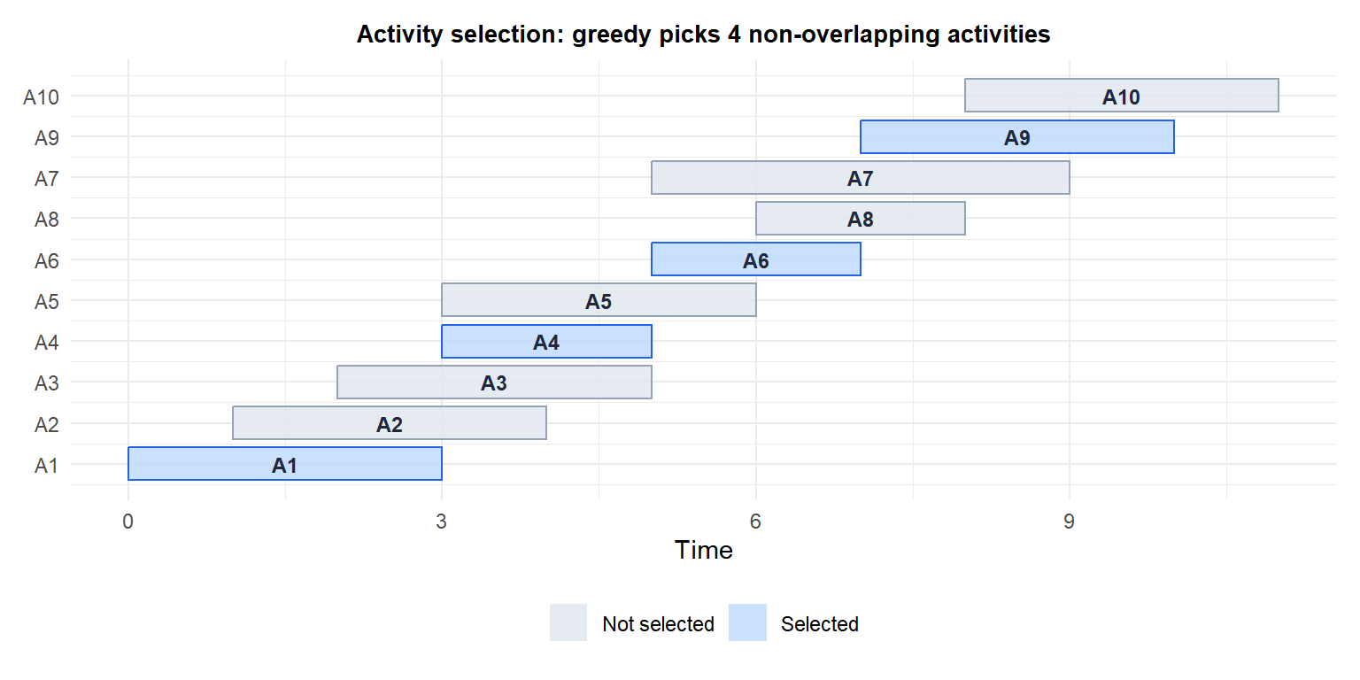
\(n\) activities with start times \(s_i\) and finish times \(f_i\). Select the maximum number of non-overlapping activities.
Greedy strategy: always select the activity that finishes earliest among those compatible with the current selection.
Why it works: choosing the activity that finishes first leaves the most remaining time for other activities. Any solution that skips the earliest-finishing compatible activity can be improved by swapping in that activity (exchange argument).
Algorithm: sort activities by finish time. Scan left to right; add each activity if it does not overlap with the last selected.
Time complexity: \(O(n \log n)\) for sorting, \(O(n)\) for the scan.
Example 2: Huffman coding
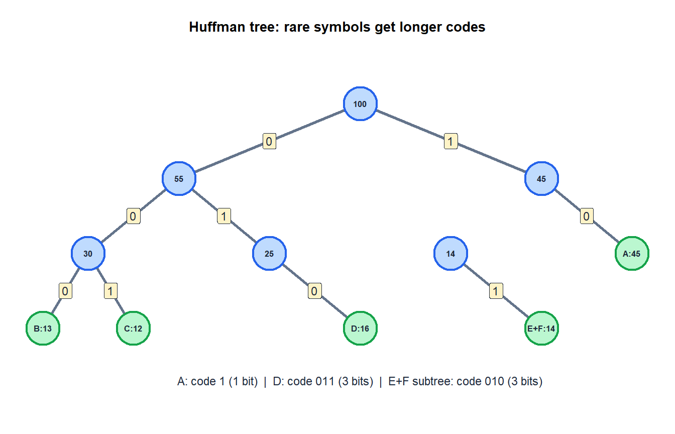
Assign binary codes to \(n\) symbols with frequencies \(f_i\) to minimize the total encoded length \(\sum_i f_i \cdot \text{depth}(i)\), where depth is the code length.
Greedy strategy: repeatedly merge the two symbols (or subtrees) with the lowest frequencies into a new subtree. The merged node’s frequency is the sum of the two children.
Why it works: the two rarest symbols should be deepest in the tree (longest codes), since their contribution \(f_i \cdot \text{depth}(i)\) to total length is minimized by giving them the longest codes. The exchange argument shows that any other assignment is no better.
Result: Huffman coding is provably optimal among all prefix-free codes. It underlies DEFLATE compression (ZIP, PNG, HTTP/2).
Example 3: minimum spanning tree (Kruskal’s algorithm)
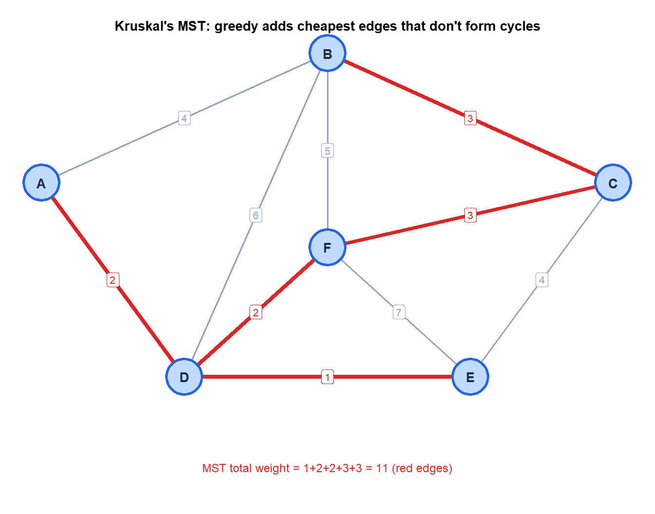
Given a connected weighted graph, find the spanning tree (subgraph connecting all vertices with no cycles) of minimum total edge weight.
Kruskal’s greedy strategy: sort all edges by weight. Add each edge to the spanning tree if it does not create a cycle.
Why it works: the cut property of spanning trees guarantees that the minimum-weight edge crossing any cut (partition of vertices into two sets) is safe to include. Each greedy edge selection satisfies this property.
Time complexity: \(O(E \log E)\) for sorting, nearly \(O(E \alpha(V))\) for cycle detection with a Union-Find data structure (\(\alpha\) is the inverse Ackermann function, effectively constant).
When greedy fails
The greedy choice property does not always hold. The classic failure: the coin change problem with non-standard denominations.
With coins \(\{1, 5, 6\}\) and target amount 10:
- Greedy (largest coin first): \(6 + 1 + 1 + 1 + 1 = 5\) coins.
- Optimal (DP): \(5 + 5 = 2\) coins.
The greedy choice (pick 6) is locally optimal but globally suboptimal. DP finds the correct answer.
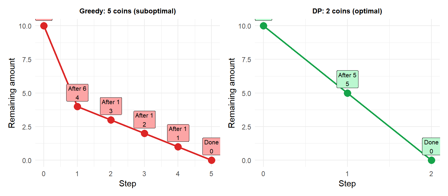
With coins \(\{1, 5, 6\}\) and target 10, greedy takes 5 coins while DP finds the optimal 2.
Greedy vs dynamic programming
| Greedy | Dynamic programming | |
|---|---|---|
| Approach | Local optimal choice at each step | Solve all subproblems, combine |
| Reconsideration | Never | No (but considers all options) |
| Correctness | Only when greedy choice property holds | Whenever optimal substructure holds |
| Time complexity | Usually \(O(n \log n)\) or \(O(n)\) | Usually \(O(n^k)\) for some \(k\) |
| Space complexity | \(O(1)\) or \(O(n)\) | \(O(n^k)\) table |
| Examples | Activity selection, Huffman, Kruskal, Dijkstra | Knapsack, LCS, edit distance, TSP |
Greedy is always preferable when it works: simpler and faster. Use DP when greedy fails due to lack of the greedy choice property.
⚠️ Proving greedy correctness requires an exchange argument
Greedy algorithms are easy to design but hard to prove correct. Never assume a greedy strategy works just because it seems intuitive. For every greedy algorithm, you must prove the greedy choice property: show that including the greedy choice in the solution does not prevent finding an optimal completion.
The standard proof template: assume an optimal solution \(OPT\) that does not make the greedy choice at step \(k\). Construct \(OPT'\) by swapping in the greedy choice. Show that \(OPT'\) is feasible and no worse than \(OPT\). Therefore, there exists an optimal solution making the greedy choice, and the greedy algorithm is correct.
Without this proof, a plausible greedy strategy can fail on specific inputs, as the coin change example shows.
💡 Greedy algorithms in R
# Activity selection
activity_selection <- function(start, finish) {
  n    <- length(start)
  idx  <- order(finish)           # sort by finish time
  sel  <- idx[1]                  # always select first
  last <- finish[idx[1]]
  for (i in 2:n) {
    j <- idx[i]
    if (start[j] >= last) {
      sel  <- c(sel, j)
      last <- finish[j]
    }
  }
  sel
}

# Kruskal MST via igraph
library(igraph)
g <- graph_from_data_frame(
  data.frame(from=c("A","A","B","B","B","C","C","D","D","E"),
             to  =c("B","D","C","D","F","E","F","E","F","F"),
             weight=c(4,2,3,6,5,4,3,1,2,7)),
  directed=FALSE
)
mst_g <- mst(g, weights=E(g)$weight)  # Kruskal internally
sum(E(mst_g)$weight)  # 11
