Convex optimization

Convex optimization is the class of problems where the objective function and feasible set are both convex. This single property has an enormous consequence: every local minimum is a global minimum. Convex problems can be solved reliably and efficiently regardless of their size, while non-convex problems are generally intractable in the worst case.

Convex sets

A set \(\mathcal{C} \subseteq \mathbb{R}^n\) is convex if the line segment between any two points in \(\mathcal{C}\) lies entirely within \(\mathcal{C}\):

\[x, y \in \mathcal{C} \implies \theta x + (1-\theta)y \in \mathcal{C} \quad \forall \theta \in [0,1]\]

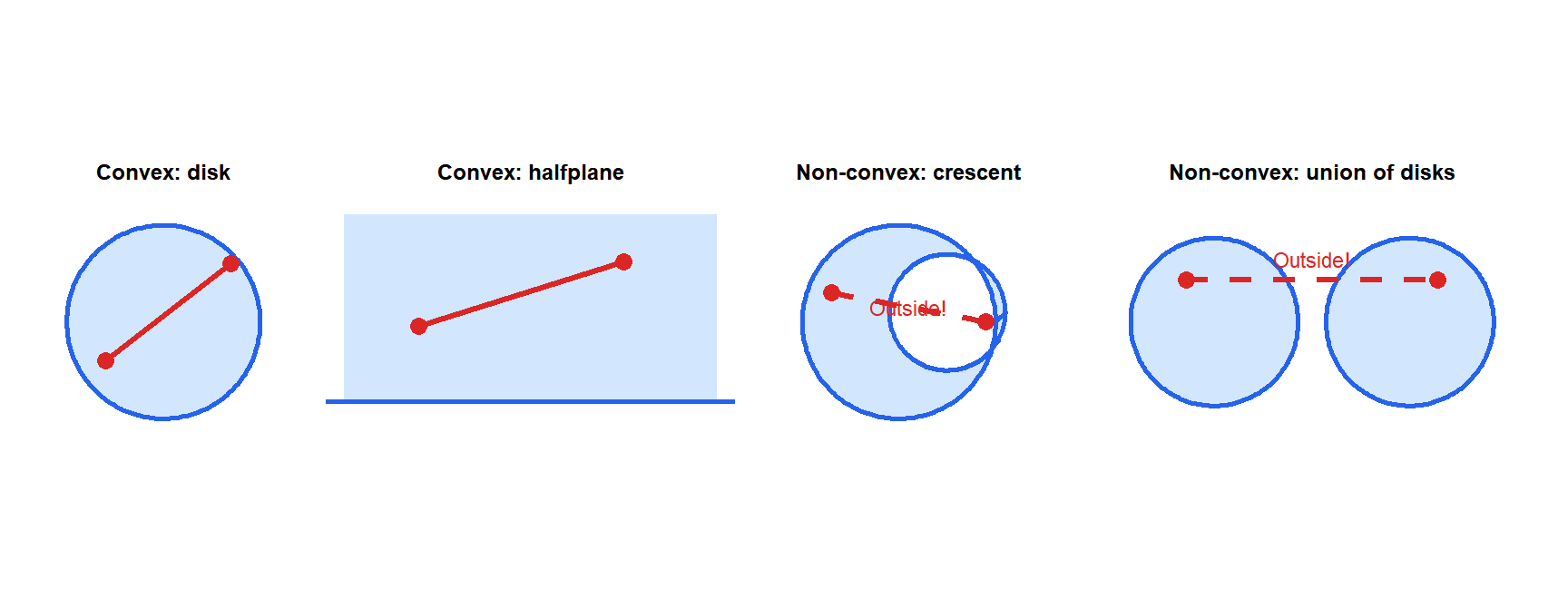
The red segment lies entirely within the convex sets (disk, halfplane) but exits the non-convex ones (crescent, union of disks). Important convex sets: halfspaces, polyhedra (intersections of halfspaces), balls, ellipsoids, cones.

Convex functions

A function \(f: \mathbb{R}^n \to \mathbb{R}\) is convex if its domain is convex and:

\[f(\theta x + (1-\theta)y) \leq \theta f(x) + (1-\theta)f(y) \quad \forall x,y,\; \theta \in [0,1]\]

Geometrically: the chord between any two points on the graph lies above (or on) the graph.

For twice-differentiable \(f\): \(f\) is convex iff \(\nabla^2 f(x) \succeq 0\) (positive semidefinite Hessian) everywhere.

Operations that preserve convexity: non-negative linear combinations, pointwise maximum, composition with affine functions. These allow building complex convex functions from simple ones.

Common convex functions:

• Quadratic: \(f(x) = x^T Q x + b^T x\) with \(Q \succeq 0\).
• Exponential: \(e^{ax}\) for any \(a\).
• Powers: \(|x|^p\) for \(p \geq 1\); \(x^p\) for \(p \geq 1\) on \(x > 0\).
• Norms: \(\|x\|_p\) for \(p \geq 1\).
• Log-sum-exp: \(\log\sum_i e^{x_i}\) (smooth approximation of max).
• Negative entropy: \(\sum_i x_i \log x_i\).

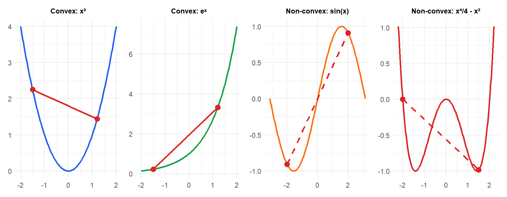
For convex functions (blue, green) the chord lies above the curve. For non-convex functions (orange, red) the chord dips below: the definition is violated.

Standard convex optimization problem

where \(f_0, f_1, \ldots, f_m\) are all convex and the equality constraints are affine. The feasible set \(\{x : f_i(x) \leq 0,\; Ax = b\}\) is convex (intersection of convex sets).

The fundamental theorem of convex optimization: any local minimum of a convex problem is a global minimum. If \(f_0\) is strictly convex, the global minimum is unique.

This is the property that makes convex optimization tractable: we do not need to worry about getting trapped in local minima. Any descent algorithm will find the global optimum.

Hierarchy of convex problem classes

Convex optimization encompasses a hierarchy of increasingly general problem classes, each with specialized solvers:

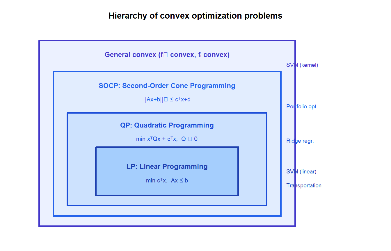
Each class is a special case of the one above. Specialized solvers exist for each level: the Simplex method for LP, active-set or interior point for QP, SOCP solvers for second-order cone constraints.

Lagrange duality and strong duality

For any optimization problem (convex or not), the Lagrange dual problem is:

\[\max_{\lambda \geq 0,\, \nu} g(\lambda, \nu), \qquad g(\lambda, \nu) = \inf_x \mathcal{L}(x, \lambda, \nu) = \inf_x \left[f_0(x) + \sum_i \lambda_i f_i(x) + \nu^T(Ax-b)\right]\]

The dual function \(g(\lambda, \nu)\) is always concave (even if the primal is non-convex) and provides a lower bound on the primal optimal value \(p^*\):

\[g(\lambda, \nu) \leq p^* \quad \forall \lambda \geq 0, \nu\]

The gap \(p^* - g(\lambda^*, \nu^*)\) is the duality gap.

Weak duality: \(d^* \leq p^*\) always. Strong duality: \(d^* = p^*\) (zero gap). Strong duality holds for convex problems under Slater’s condition: there exists a strictly feasible point \(\hat{x}\) with \(f_i(\hat{x}) < 0\) for all inequality constraints.

Under strong duality, the KKT conditions are both necessary and sufficient for optimality. Solving the dual is sometimes easier than the primal: the SVM dual is a quadratic program that leads naturally to the kernel trick and sparse solutions.

KKT conditions for convex problems

For convex problems satisfying Slater’s condition, the KKT conditions are necessary and sufficient for global optimality. A point \(x^*\) is the global optimum if and only if there exist \(\lambda^* \geq 0\) and \(\nu^*\) such that:

• Primal feasibility: \(f_i(x^*) \leq 0\), \(Ax^* = b\).
• Dual feasibility: \(\lambda_i^* \geq 0\).
• Complementary slackness: \(\lambda_i^* f_i(x^*) = 0\).
• Stationarity: \(\nabla f_0(x^*) + \sum_i \lambda_i^* \nabla f_i(x^*) + A^T\nu^* = 0\).

This is the clean version of the KKT result: for non-convex problems, KKT is only necessary. For convex problems under Slater’s condition, it characterizes the global optimum completely.

library(CVXR)

# Lasso (L1-regularized least squares): convex but non-smooth
n <- 50; p <- 20
X <- matrix(rnorm(n*p), n, p)
y <- rnorm(n)
beta <- Variable(p)
lambda <- 0.1

prob <- Problem(Minimize(sum_squares(X %*% beta - y) + lambda*sum(abs(beta))))
solve(prob)
beta$value

# Portfolio optimization: minimize variance subject to return constraint
w <- Variable(p, nonneg=TRUE)           # weights >= 0
Sigma <- cov(matrix(rnorm(n*p), n, p)) # covariance matrix
mu <- rnorm(p, 0.05, 0.02)             # expected returns
target_return <- 0.04

prob <- Problem(Minimize(quad_form(w, Sigma)),
                list(sum(w) == 1,
                     t(mu) %*% w >= target_return))
solve(prob)

# Linear program
c_obj <- c(5, 4)
A_mat <- rbind(c(1,2), c(2,1))
b_rhs <- c(8, 10)
x <- Variable(2, nonneg=TRUE)
prob <- Problem(Maximize(t(c_obj) %*% x),
                list(A_mat %*% x <= b_rhs))
solve(prob)