Support vector machines (SVM)
Support Vector Machines find the hyperplane that separates two classes with the largest possible margin. Points closest to the hyperplane (the support vectors) are the only ones that determine its position: all other training points are irrelevant. The kernel trick extends SVMs to nonlinear boundaries by implicitly mapping data to a high-dimensional space.
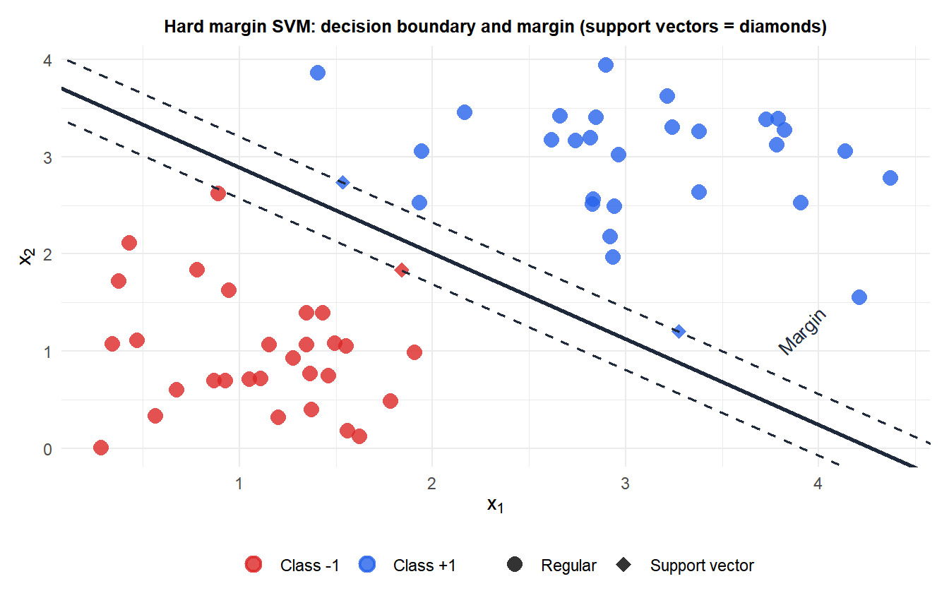
Hard margin SVM
For linearly separable data with labels \(y_i \in \{-1, +1\}\), the decision boundary is a hyperplane \(\mathbf{w}^T\mathbf{x} + b = 0\). Points with \(y_i = +1\) should satisfy \(\mathbf{w}^T\mathbf{x}_i + b \geq +1\) and points with \(y_i = -1\) should satisfy \(\mathbf{w}^T\mathbf{x}_i + b \leq -1\). Combining: \(y_i(\mathbf{w}^T\mathbf{x}_i + b) \geq 1\) for all \(i\).
The margin width is \(2/\|\mathbf{w}\|\). Maximizing the margin is equivalent to minimizing \(\|\mathbf{w}\|^2\):
\[\min_{\mathbf{w},b} \frac{1}{2}\|\mathbf{w}\|^2 \quad \text{s.t.} \quad y_i(\mathbf{w}^T\mathbf{x}_i + b) \geq 1 \quad \forall i\]
This is a convex quadratic program. The KKT conditions give the dual problem, and only the training points where \(y_i(\mathbf{w}^T\mathbf{x}_i + b) = 1\) (on the margin boundary) have nonzero dual variables \(\alpha_i > 0\): these are the support vectors. All other points are irrelevant to the solution. This sparsity is a key property: predictions use only the support vectors.
Soft margin SVM
Real data is rarely linearly separable. The soft margin SVM introduces slack variables \(\xi_i \geq 0\) that allow points to violate the margin constraint:
\[\min_{\mathbf{w},b,\boldsymbol{\xi}} \frac{1}{2}\|\mathbf{w}\|^2 + C\sum_{i=1}^n \xi_i \quad \text{s.t.} \quad y_i(\mathbf{w}^T\mathbf{x}_i + b) \geq 1 - \xi_i,\quad \xi_i \geq 0\]
The parameter \(C > 0\) controls the tradeoff:
- Large \(C\): penalizes margin violations heavily. Smaller margin but fewer misclassifications on training data. Prone to overfitting.
- Small \(C\): tolerates more violations. Wider margin, more regularized. Prone to underfitting.
\(C\) is the most important hyperparameter and must be selected by cross-validation. The support vectors are now points that either lie on the margin boundary (\(\xi_i = 0\), \(\alpha_i > 0\)) or violate it (\(\xi_i > 0\)): the fraction of support vectors typically increases as \(C\) decreases.
The dual problem and kernels
The Lagrangian dual of the soft margin problem is:
\[\max_{\boldsymbol{\alpha}} \sum_i \alpha_i - \frac{1}{2}\sum_{i,j}\alpha_i\alpha_j y_i y_j \mathbf{x}_i^T\mathbf{x}_j \quad \text{s.t.} \quad 0 \leq \alpha_i \leq C,\quad \sum_i \alpha_i y_i = 0\]
The key observation: the objective depends on the data only through inner products \(\mathbf{x}_i^T\mathbf{x}_j\). The prediction for a new point also uses only inner products:
\[\hat{y}(\mathbf{x}) = \text{sign}\!\left(\sum_{i \in SV} \alpha_i y_i \mathbf{x}_i^T\mathbf{x} + b\right)\]
The kernel trick: replace every inner product \(\mathbf{x}_i^T\mathbf{x}_j\) with a kernel function \(K(\mathbf{x}_i, \mathbf{x}_j) = \phi(\mathbf{x}_i)^T\phi(\mathbf{x}_j)\) where \(\phi\) is an implicit feature map. This allows the SVM to operate in a very high (or infinite) dimensional feature space without ever computing \(\phi(\mathbf{x})\) explicitly.
Common kernels
| Kernel | Formula | When to use |
|---|---|---|
| Linear | \(K(\mathbf{x},\mathbf{x}') = \mathbf{x}^T\mathbf{x}'\) | Linearly separable, high \(p\) |
| Polynomial | \(K(\mathbf{x},\mathbf{x}') = (\mathbf{x}^T\mathbf{x}' + c)^d\) | Polynomial interactions |
| RBF/Gaussian | \(K(\mathbf{x},\mathbf{x}') = e^{-\gamma\|\mathbf{x}-\mathbf{x}'\|^2}\) | General nonlinear, most common |
| Sigmoid | \(K(\mathbf{x},\mathbf{x}') = \tanh(\kappa\mathbf{x}^T\mathbf{x}' + c)\) | Neural network-like |
The RBF kernel with bandwidth \(\gamma\) is the most widely used. Smaller \(\gamma\): smoother boundary (farther points influence each other). Larger \(\gamma\): each training point influences only its immediate neighborhood, leading to overfitting.
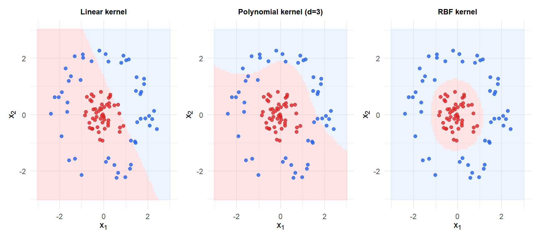
On circular data (not linearly separable), the linear kernel fails completely. The polynomial kernel captures some nonlinearity. The RBF kernel correctly learns the circular boundary.
Hyperparameter tuning
Two key hyperparameters for RBF-SVM: \(C\) and \(\gamma\). They interact: large \(\gamma\) with large \(C\) overfits; small \(\gamma\) with small \(C\) underfits. The standard approach is a 2D grid search with cross-validation:
- \(C\) grid: \(\{0.01, 0.1, 1, 10, 100, 1000\}\)
- \(\gamma\) grid: \(\{0.001, 0.01, 0.1, 1, 10\}\)
A heuristic starting point for \(\gamma\): \(1/(p \cdot \text{Var}(\mathbf{X}))\) where \(p\) is the number of features.
⚠️ SVM scales poorly with large n
Training SVM requires solving a quadratic program with \(n\) variables. Naive QP solvers have \(O(n^3)\) complexity. Sequential Minimal Optimization (SMO), the standard algorithm in libsvm, reduces this to roughly \(O(n^2)\) but can still be slow for \(n > 100{,}000\).
For large datasets: use a linear SVM (much faster, \(O(n)\) with stochastic gradient methods) or switch to gradient boosting / neural networks which scale better. The kernel trick is powerful but computationally expensive at prediction time too: predictions require evaluating \(K(\mathbf{x}, \mathbf{x}_i)\) for all support vectors.
💡 SVM in R
library(e1071)

# Linear SVM
fit_lin <- svm(y ~ ., data=df_train, kernel="linear", cost=1)

# RBF SVM
fit_rbf <- svm(y ~ ., data=df_train, kernel="radial",
               cost=10, gamma=0.1)

# Grid search for C and gamma
tune_result <- tune(svm, y ~ ., data=df_train,
                    kernel="radial",
                    ranges=list(cost=10^(-1:3), gamma=10^(-3:1)))
best_model <- tune_result$best.model
summary(tune_result)

# Predictions and probabilities
predict(fit_rbf, newdata=df_test)
predict(fit_rbf, newdata=df_test, decision.values=TRUE)

# Support vector regression (SVR)
fit_svr <- svm(y ~ ., data=df_train, type="eps-regression",
               kernel="radial", epsilon=0.1)
