HOME

Simple linear regression

Simple linear regression models the linear relationship between a response variable $y$ and a single predictor $x$ by fitting a straight line through the data. It is the foundation of regression analysis: every multiple regression, logistic regression, and regularized model builds on these concepts.

The model

\[y_i = \beta_0 + \beta_1 x_i + \varepsilon_i, \qquad \varepsilon_i \sim N(0, \sigma^2)\]

$\beta_0$: intercept. The expected value of $y$ when $x = 0$.
$\beta_1$: slope. The expected change in $y$ for a one-unit increase in $x$.
$\varepsilon_i$: error term. Captures everything that affects $y$ beyond $x$: measurement error, omitted variables, inherent randomness.

The model makes four assumptions (LINE): Linearity, Independence of errors, Normality of errors, Equal variance (homoscedasticity). These are tested in the diagnostics post.

OLS estimation

Ordinary Least Squares (OLS) finds $\hat{\beta}_0$ and $\hat{\beta}_1$ that minimize the sum of squared residuals:

\[\text{SSE} = \sum_{i=1}^n (y_i - \hat{\beta}_0 - \hat{\beta}_1 x_i)^2\]

Taking derivatives and setting them to zero gives the closed-form estimators:

\[\hat{\beta}_1 = \frac{\sum_{i=1}^n (x_i - \bar{x})(y_i - \bar{y})}{\sum_{i=1}^n (x_i - \bar{x})^2} = r_{xy} \cdot \frac{S_y}{S_x}\]

\[\hat{\beta}_0 = \bar{y} - \hat{\beta}_1 \bar{x}\]

where $r_{xy}$ is the Pearson correlation, $S_y$ and $S_x$ are the sample standard deviations. The regression line always passes through the point of means $(\bar{x}, \bar{y})$.

The connection with correlation: $\hat{\beta}_1 = 0$ iff $r_{xy} = 0$. Testing $H_0: \beta_1 = 0$ is equivalent to testing $H_0: \rho = 0$.

Example: advertising spend and sales

A company tracks weekly TV advertising spend (thousands of €) and weekly sales (thousands of units) over 50 weeks.

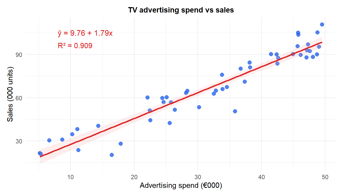
Scatter plot of advertising spend vs sales with fitted regression line and confidence band

Each additional €1,000 of TV advertising is associated with approximately 1.79 thousand extra units sold. The intercept (9.76) represents baseline sales with zero advertising. $R^2 = $ 0.909 means 90.9% of the variation in sales is explained by advertising spend.

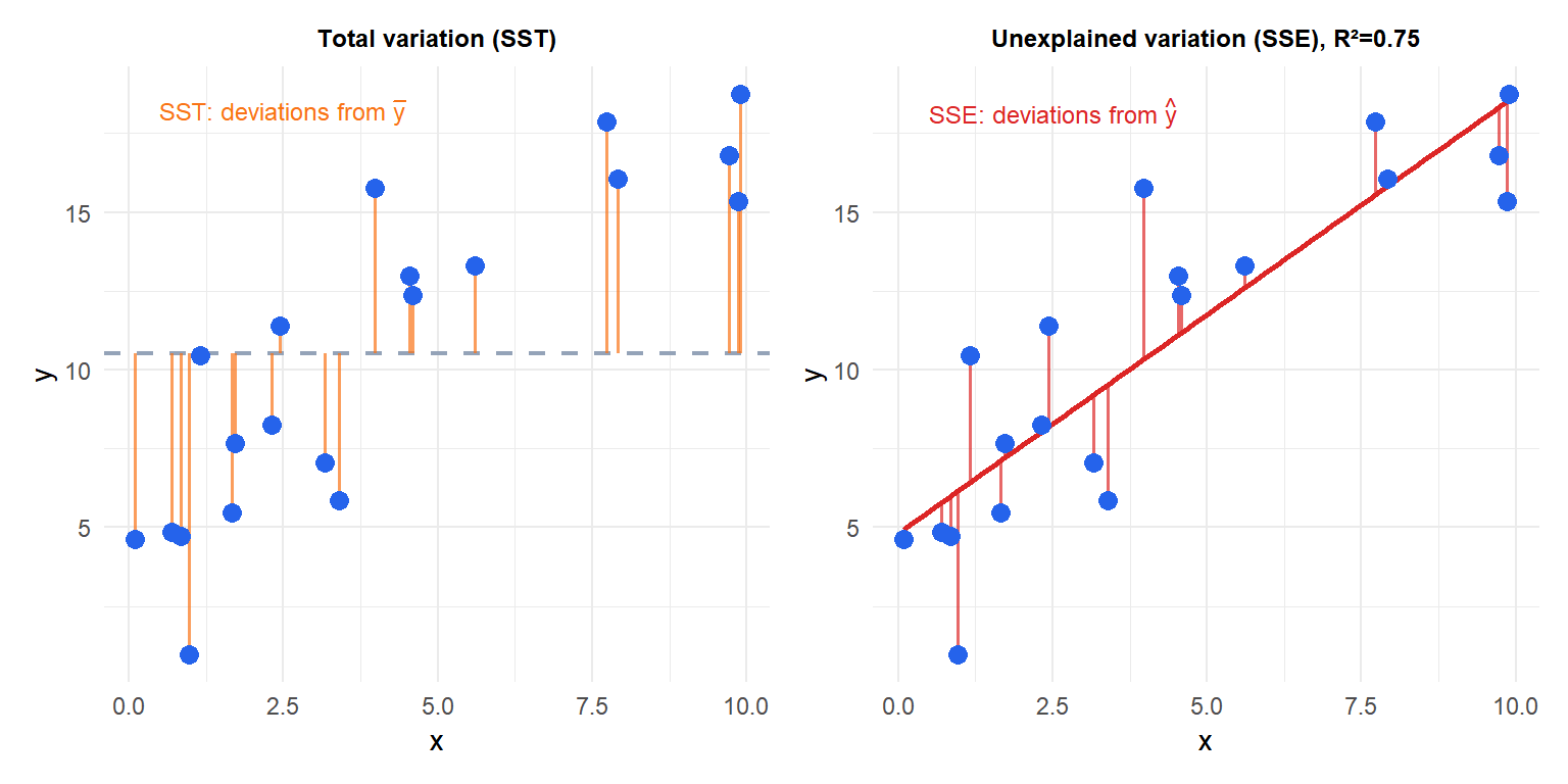
Goodness of fit: R²

$R^2$ measures the proportion of variance in $y$ explained by the model:

\[R^2 = 1 - \frac{\text{SSE}}{\text{SST}} = 1 - \frac{\sum(y_i - \hat{y}_i)^2}{\sum(y_i - \bar{y})^2}\]

$R^2 \in [0,1]$. An $R^2$ of 0.70 means 70% of the variance in $y$ is explained by $x$; the remaining 30% is unexplained noise. In simple linear regression, $R^2 = r_{xy}^2$.

Two panels showing SST (total variation) and SSE (unexplained variation) for the same regression to illustrate R squared

Inference on the slope

Under the model assumptions, $\hat{\beta}_1$ is normally distributed:

\[\hat{\beta}_1 \sim N\!\left(\beta_1,\; \frac{\sigma^2}{\sum(x_i-\bar{x})^2}\right)\]

Since $\sigma^2$ is unknown, we estimate it with $\hat{\sigma}^2 = \text{SSE}/(n-2)$ and use the $t$-distribution:

\[t = \frac{\hat{\beta}_1 - 0}{\widehat{\text{SE}}(\hat{\beta}_1)} \sim t(n-2) \quad \text{under } H_0: \beta_1 = 0\]

A $(1-\alpha)$ confidence interval for $\beta_1$:

\[\hat{\beta}_1 \pm t_{\alpha/2, n-2} \cdot \widehat{\text{SE}}(\hat{\beta}_1)\]

A significant $t$-test ($p < 0.05$) means $x$ is a statistically significant predictor of $y$: the observed slope is unlikely to arise by chance if $\beta_1 = 0$.

⚠️ Statistical significance does not imply practical importance

A very large sample can produce a statistically significant slope that is practically negligible. An increase of $\hat{\beta}_1 = 0.001$ units per €1,000 of advertising may be significant at $p < 0.001$ with $n = 10{,}000$ observations, but it is commercially irrelevant.

Always report the effect size (the slope itself and its confidence interval) alongside the p-value. The confidence interval communicates both the direction and the plausible magnitude of the effect.

Prediction

For a new observation at $x_\text{new}$, the model produces two types of intervals:

Confidence interval for the mean response: uncertainty about the average $y$ at $x_\text{new}$ across the population.

Prediction interval for a new observation: wider, because it adds the individual error $\varepsilon$ on top of the uncertainty about the mean.

\[\hat{y}_\text{new} \pm t_{\alpha/2, n-2} \cdot \hat{\sigma}\sqrt{1 + \frac{1}{n} + \frac{(x_\text{new}-\bar{x})^2}{\sum(x_i-\bar{x})^2}}\]

Both intervals widen as $x_\text{new}$ moves away from $\bar{x}$: extrapolation is increasingly unreliable.

💡 Simple linear regression in R

fit <- lm(sales ~ spend, data = df)
summary(fit)         # coefficients, t-tests, R²
confint(fit)         # 95% CIs for beta0 and beta1
predict(fit, newdata = data.frame(spend = 30),
        interval = "confidence")   # CI for mean response
predict(fit, newdata = data.frame(spend = 30),
        interval = "prediction")   # PI for new observation