Principal component analysis (PCA)
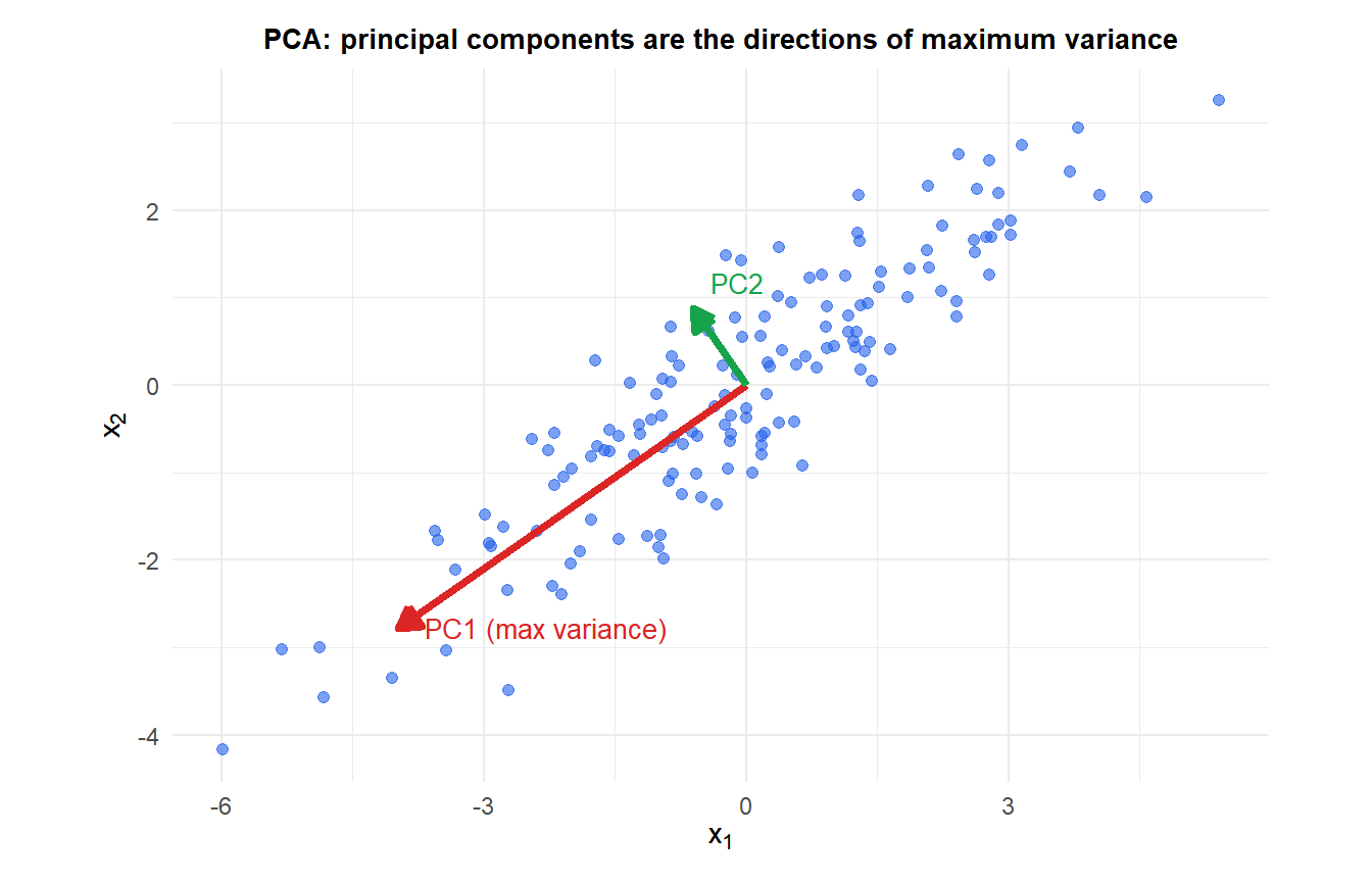
Principal Component Analysis (PCA) finds a lower-dimensional representation of the data that captures as much variance as possible. It does this by rotating the coordinate system to align with the directions of maximum variance in the data. The result is a set of uncorrelated components, ordered by the amount of variance they explain.
What PCA does geometrically
Given \(n\) observations of \(p\) variables, PCA finds a sequence of orthogonal directions \(\mathbf{v}_1, \mathbf{v}_2, \ldots, \mathbf{v}_p\) (the principal components) such that:
- \(\mathbf{v}_1\) is the direction of maximum variance in the data.
- \(\mathbf{v}_2\) is the direction of maximum variance in the subspace orthogonal to \(\mathbf{v}_1\).
- And so on.
The projection of the data onto \(\mathbf{v}_k\) gives the scores \(\mathbf{z}_k = \mathbf{X}\mathbf{v}_k\): the coordinates of each observation in the new coordinate system. The directions \(\mathbf{v}_k\) are called loadings: they tell you how much each original variable contributes to each component.
Mathematical derivation
Center the data: \(\tilde{\mathbf{X}} = \mathbf{X} - \bar{\mathbf{X}}\). The sample covariance matrix is:
\[\mathbf{S} = \frac{1}{n-1}\tilde{\mathbf{X}}^T\tilde{\mathbf{X}}\]
The principal components are the eigenvectors of \(\mathbf{S}\):
\[\mathbf{S}\mathbf{v}_k = \lambda_k \mathbf{v}_k\]
where \(\lambda_k\) is the variance explained by the \(k\)-th component. The eigenvectors are orthonormal (\(\mathbf{v}_j^T\mathbf{v}_k = 0\) for \(j \neq k\), \(\|\mathbf{v}_k\|=1\)) and ordered by decreasing eigenvalue \(\lambda_1 \geq \lambda_2 \geq \cdots \geq \lambda_p \geq 0\).
Connection to SVD: the singular value decomposition of \(\tilde{\mathbf{X}} = \mathbf{U}\mathbf{D}\mathbf{V}^T\) gives immediately:
\[\tilde{\mathbf{X}}^T\tilde{\mathbf{X}} = \mathbf{V}\mathbf{D}^2\mathbf{V}^T\]
The right singular vectors \(\mathbf{V}\) are the principal component loadings, and the singular values \(d_k\) relate to eigenvalues via \(\lambda_k = d_k^2/(n-1)\). Computing PCA via SVD is numerically more stable than eigendecomposition of \(\mathbf{S}\) when \(p\) is large or some variables are nearly collinear.
Covariance vs correlation PCA
PCA on the covariance matrix preserves the original scale: variables with large variance dominate the components. PCA on the correlation matrix (equivalent to standardizing each variable to unit variance first) gives equal weight to all variables regardless of their scale.
Always standardize when variables are measured in different units (e.g., height in cm and weight in kg). When all variables are on the same scale (e.g., gene expression counts), covariance PCA is appropriate and preserves meaningful differences in variance.
Choosing the number of components
The proportion of variance explained by component \(k\):
\[\text{PVE}_k = \frac{\lambda_k}{\sum_{j=1}^p \lambda_j}\]
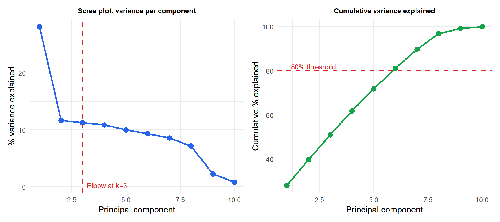
Scree plot: plot \(\lambda_k\) (or \(\text{PVE}_k\)) vs \(k\). Look for the “elbow” where the curve flattens. Components to the left of the elbow capture most of the structure; those to the right capture noise.
Kaiser criterion: retain components with \(\lambda_k > 1\) (for correlation PCA: components that explain more than a single original variable).
Cumulative variance threshold: retain enough components to explain 80-90% of total variance.
The biplot
A biplot overlays the scores (observations in PC space) and the loadings (original variables as arrows) in the same plot. It allows simultaneous interpretation of both:
- Observations close together have similar profiles.
- Variables (arrows) pointing in the same direction are positively correlated; opposite directions are negatively correlated; perpendicular arrows are uncorrelated.
- Arrow length indicates how much of the variable’s variance is captured by the two components shown.
- Observation close to an arrow scores high on that variable.
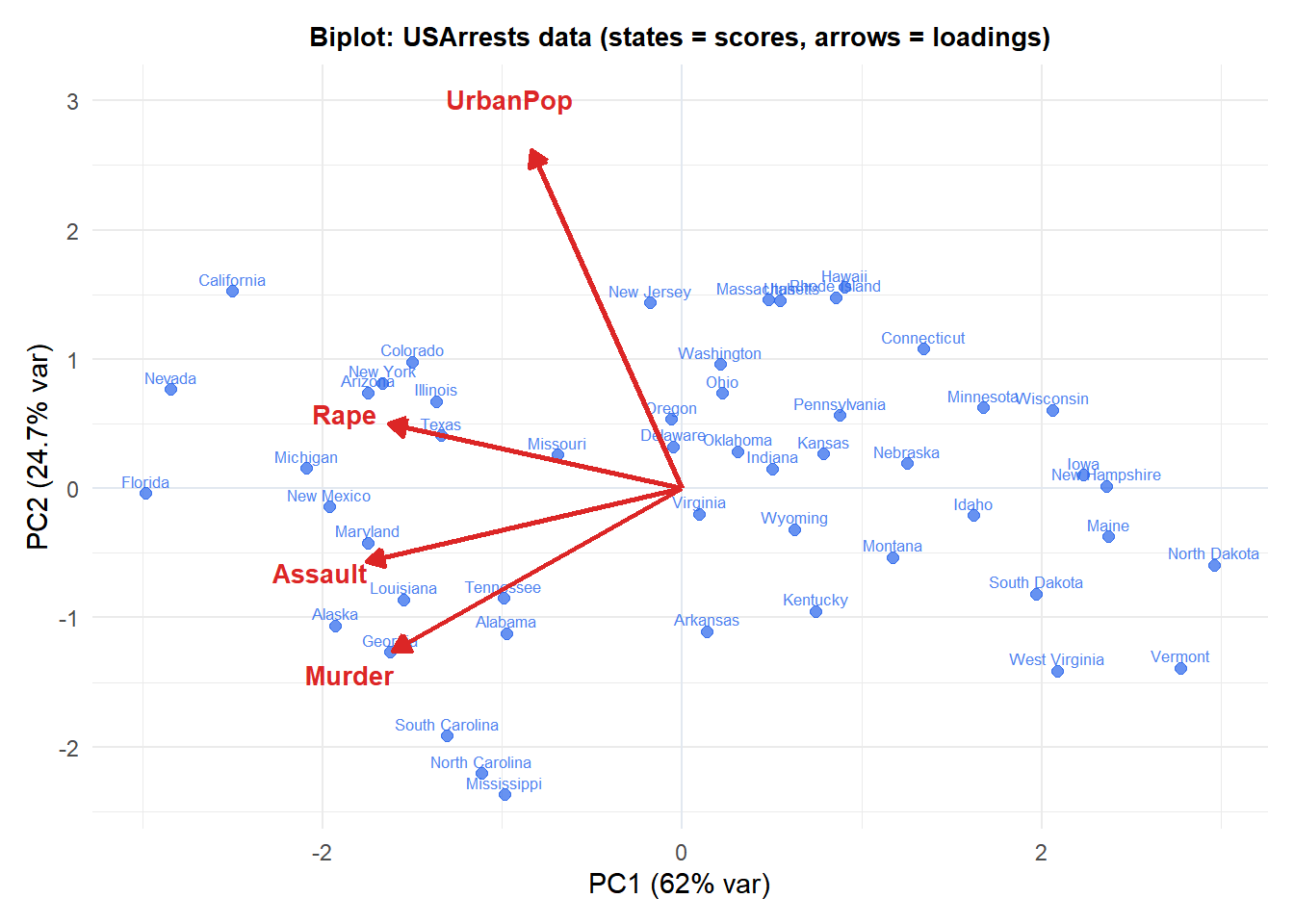
PC1 (horizontal) separates high-crime states (right) from low-crime states (left): Murder, Assault and Rape all point right, meaning PC1 is a general crime index. PC2 (vertical) is driven mainly by UrbanPop: states with high urban population score high on PC2 regardless of crime rates.
PCA vs LDA
Both PCA and LDA project data to a lower-dimensional space, but with different objectives:
- PCA: unsupervised. Maximizes total variance of the projected data. Ignores class labels. Useful for visualization, noise reduction, and preprocessing.
- LDA: supervised. Maximizes between-class variance relative to within-class variance. Uses class labels. Useful when the goal is classification or finding directions that separate known classes.
If the directions of maximum variance happen to be the same as the directions that separate classes, PCA and LDA agree. When the most variable direction is within-class noise (e.g., individuals vary a lot within each class but classes differ in a low-variance direction), PCA fails to find the discriminative structure and LDA is needed.
⚠️ PCA does not guarantee interpretable components
Each principal component is a linear combination of all original variables. Even if PC1 captures 60% of variance, it may be a weighted average of 20 variables with similar loadings: there is no guarantee that it corresponds to a meaningful scientific concept.
Techniques like sparse PCA (impose L1 penalty on loadings to force most to zero) and varimax rotation (rotate components to maximize the simplicity of the loading structure) can improve interpretability, at the cost of losing the maximum-variance optimality property.
💡 PCA in R
# Fit PCA
pca <- prcomp(X, center=TRUE, scale.=TRUE)
summary(pca)            # variance explained per component
pca$rotation            # loadings (eigenvectors)
pca$x                   # scores (projected data)

# Scree plot
plot(pca, type="l")

# Biplot
biplot(pca, scale=0)

# Choose number of components
cumsum(pca$sdev^2) / sum(pca$sdev^2)  # cumulative PVE

# Project new data onto existing PCA
predict(pca, newdata=X_new)

# Sparse PCA for interpretable loadings
library(sparsepca)
spca <- spca(X, k=3, alpha=1e-3, beta=1e-3)
