Multiple linear regression
Multiple linear regression extends simple linear regression to \(k\) predictors. Each coefficient measures the effect of one predictor while holding all others constant, a crucial distinction from simple regression where each coefficient also absorbs the effects of omitted variables.
The model
\[y_i = \beta_0 + \beta_1 x_{i1} + \beta_2 x_{i2} + \cdots + \beta_k x_{ik} + \varepsilon_i, \qquad \varepsilon_i \sim N(0, \sigma^2)\]
In matrix form, with \(\mathbf{y} \in \mathbb{R}^n\), design matrix \(\mathbf{X} \in \mathbb{R}^{n \times (k+1)}\) (first column all ones), and \(\boldsymbol{\beta} \in \mathbb{R}^{k+1}\):
\[\mathbf{y} = \mathbf{X}\boldsymbol{\beta} + \boldsymbol{\varepsilon}, \qquad \boldsymbol{\varepsilon} \sim N(\mathbf{0}, \sigma^2 \mathbf{I})\]
The OLS estimator minimizes \(\|\mathbf{y} - \mathbf{X}\boldsymbol{\beta}\|^2\) and has the closed-form solution:
\[\hat{\boldsymbol{\beta}} = (\mathbf{X}^T\mathbf{X})^{-1}\mathbf{X}^T\mathbf{y}\]
This requires \(\mathbf{X}^T\mathbf{X}\) to be invertible: the columns of \(\mathbf{X}\) must be linearly independent (no perfect multicollinearity). The fitted values are \(\hat{\mathbf{y}} = \mathbf{X}\hat{\boldsymbol{\beta}} = \mathbf{H}\mathbf{y}\) where \(\mathbf{H} = \mathbf{X}(\mathbf{X}^T\mathbf{X})^{-1}\mathbf{X}^T\) is the hat matrix.
Gauss-Markov theorem: under linearity, independence, homoscedasticity, and zero mean errors (without requiring normality), OLS is BLUE: the Best Linear Unbiased Estimator. No other linear unbiased estimator has lower variance.
Interpreting coefficients
Each \(\hat{\beta}_j\) measures the expected change in \(y\) for a one-unit increase in \(x_j\), holding all other predictors constant. This partial effect is fundamentally different from a simple regression slope, which also captures the correlation between \(x_j\) and the other predictors.
\[\widehat{\text{Price}} = 50{,}000 + 200 \cdot \text{Size} + 10{,}000 \cdot \text{Bedrooms} - 1{,}000 \cdot \text{Age}\]
- Size coefficient (200): each additional m² adds €200 to the predicted price, keeping bedrooms and age fixed.
- Bedrooms coefficient (10,000): each additional bedroom adds €10,000, keeping size and age fixed. Note that this holds size constant: a larger house that happens to have more bedrooms does not get double-counted.
- Age coefficient ($-$1,000): each additional year reduces price by €1,000, keeping size and bedrooms fixed.
Goodness of fit
R² and adjusted R²
\(R^2 = 1 - \text{SSE}/\text{SST}\) always increases when a predictor is added, even if that predictor is pure noise. Adjusted \(R^2\) penalizes for the number of predictors \(k\):
\[\bar{R}^2 = 1 - \frac{\text{SSE}/(n-k-1)}{\text{SST}/(n-1)} = 1 - (1-R^2)\frac{n-1}{n-k-1}\]
Adjusted \(R^2\) can decrease when an irrelevant predictor is added. Use \(R^2\) to report explained variance; use adjusted \(R^2\) or AIC/BIC for model selection.
F-test for overall significance
Tests \(H_0: \beta_1 = \beta_2 = \cdots = \beta_k = 0\) (no predictor is useful) vs \(H_1\): at least one \(\beta_j \neq 0\):
\[F = \frac{(\text{SST}-\text{SSE})/k}{\text{SSE}/(n-k-1)} = \frac{\text{MSR}}{\text{MSE}} \sim F(k, n-k-1) \text{ under } H_0\]
A significant F-test means the model as a whole is useful. Individual t-tests then identify which predictors contribute.
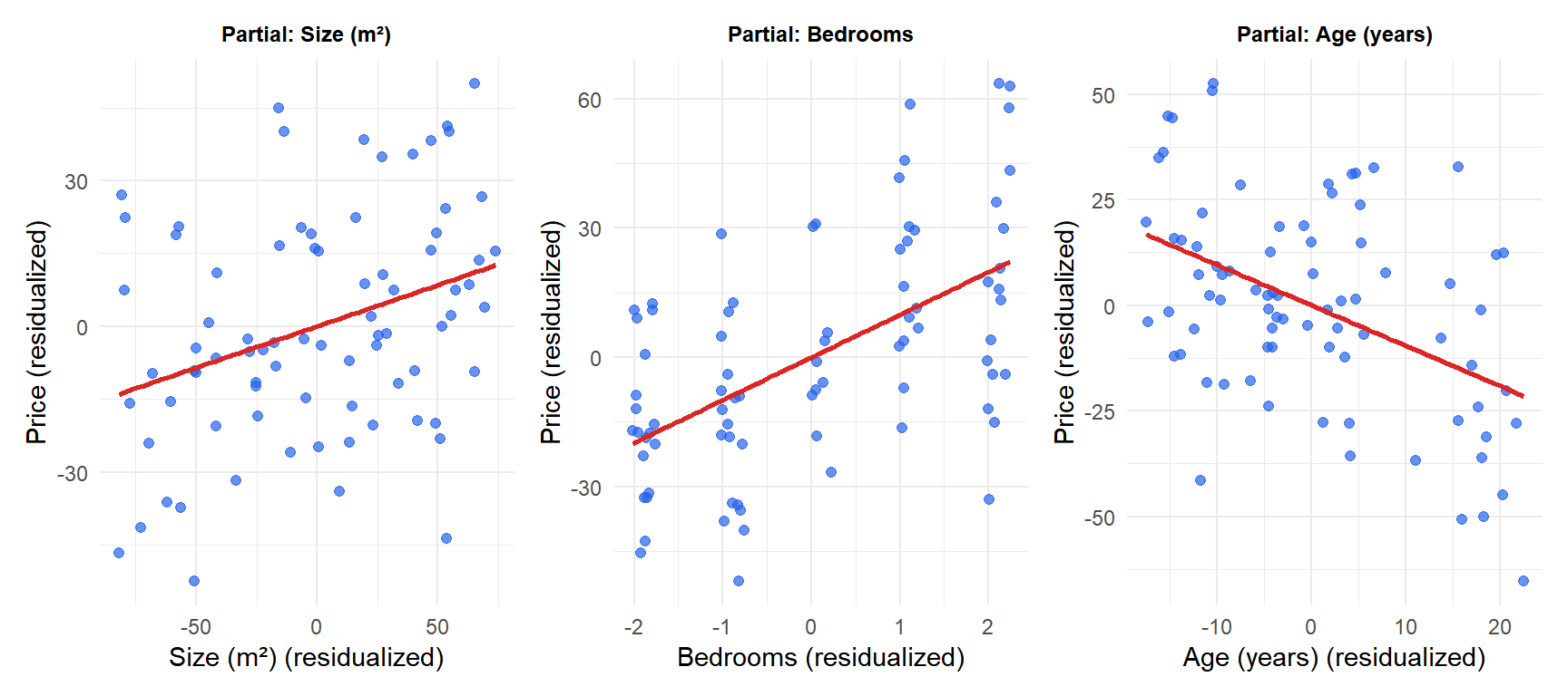
Partial regression plots show the relationship between each predictor and the response after removing the effects of all other predictors. The slope in each panel equals the corresponding OLS coefficient: the effect of size, bedrooms, and age each holding the others constant.
Multicollinearity
When predictors are highly correlated, \(\mathbf{X}^T\mathbf{X}\) becomes nearly singular: coefficient estimates are unstable with large standard errors. The predictors share credit for explaining \(y\), making it impossible to isolate their individual effects.
Variance Inflation Factor (VIF) quantifies multicollinearity for each predictor \(j\):
\[\text{VIF}_j = \frac{1}{1 - R_j^2}\]
where \(R_j^2\) is the \(R^2\) from regressing \(x_j\) on all other predictors. A \(\text{VIF}_j > 10\) (some use 5) indicates problematic multicollinearity.
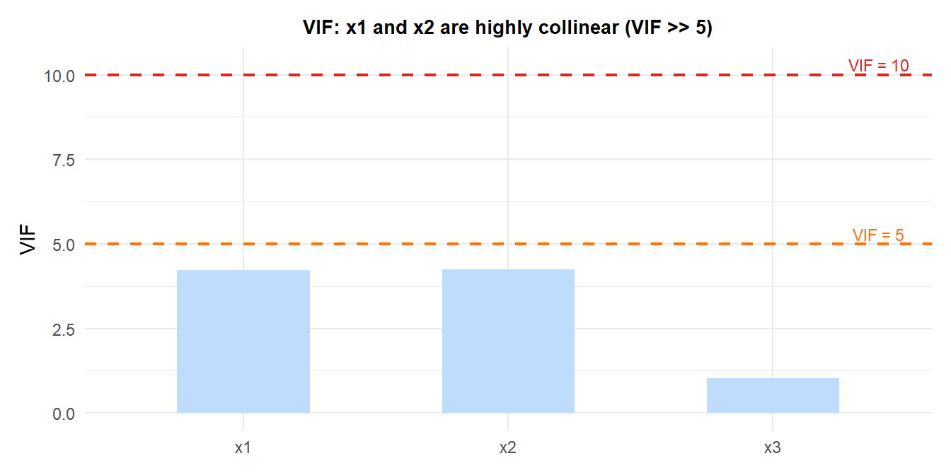
When VIF is high for predictors \(x_1\) and \(x_2\), the individual coefficients \(\hat{\beta}_1\) and \(\hat{\beta}_2\) have large standard errors and may even have the wrong sign, while their sum \(\hat{\beta}_1 + \hat{\beta}_2\) is estimated accurately. Solutions: remove one of the collinear predictors, combine them (e.g., average), or use Ridge regression.
⚠️ Adding predictors always increases R² but not model quality
Every predictor added to a model will increase (or at worst not change) \(R^2\), even if it is pure random noise. With \(n=20\) observations and \(k=19\) predictors, \(R^2 = 1\) by construction, but the model predicts nothing useful on new data.
Always use adjusted \(R^2\), AIC, or BIC for comparing models with different numbers of predictors. Better still, evaluate on held-out data via cross-validation: only improvements that generalize to new data are real.
💡 Multiple linear regression in R
fit <- lm(price ~ size + bedrooms + age, data = df)
summary(fit)             # coefficients, t-tests, F-test, R² and adjusted R²
confint(fit)             # 95% CIs for all coefficients
anova(fit)               # ANOVA table

# Multicollinearity
library(car)
vif(fit)                 # VIF for each predictor; > 5 is concerning

# Partial regression plots
avPlots(fit)

# Model comparison
AIC(fit1, fit2)
BIC(fit1, fit2)
