Lasso regression
Lasso (Least Absolute Shrinkage and Selection Operator) adds an \(L_1\) penalty to the OLS objective. The key property that distinguishes it from Ridge: the \(L_1\) penalty is not differentiable at zero, which forces some coefficients to exactly zero. Lasso is therefore simultaneously a regularization method and a variable selection method.
Objective function
\[\hat{\boldsymbol{\beta}}^L = \arg\min_{\boldsymbol{\beta}} \|\mathbf{y} - \mathbf{X}\boldsymbol{\beta}\|_2^2 + \lambda\|\boldsymbol{\beta}\|_1 = \arg\min_{\boldsymbol{\beta}} \|\mathbf{y} - \mathbf{X}\boldsymbol{\beta}\|_2^2 + \lambda\sum_{j=1}^p |\beta_j|\]
There is no closed-form solution because \(|\beta_j|\) is not differentiable at \(\beta_j = 0\). The subdifferential of \(|\beta_j|\) at zero is the interval \([-1, 1]\), which allows the solution to sit exactly at zero without the gradient condition being violated.
Why L1 produces exact zeros: soft-thresholding
For the orthonormal design case (\(\mathbf{X}^T\mathbf{X} = \mathbf{I}\)), the Lasso solution has a closed form: the soft-thresholding operator:
\[\hat{\beta}_j^L = \text{sign}(\hat{\beta}_j^{\text{OLS}}) \cdot \max(|\hat{\beta}_j^{\text{OLS}}| - \lambda/2,\; 0)\]
This shifts every OLS coefficient toward zero by \(\lambda/2\). If \(|\hat{\beta}_j^{\text{OLS}}| \leq \lambda/2\), the coefficient is set to exactly zero. Compare with Ridge, which uses a multiplicative shrinkage factor \(1/(1+\lambda)\) that never reaches zero.
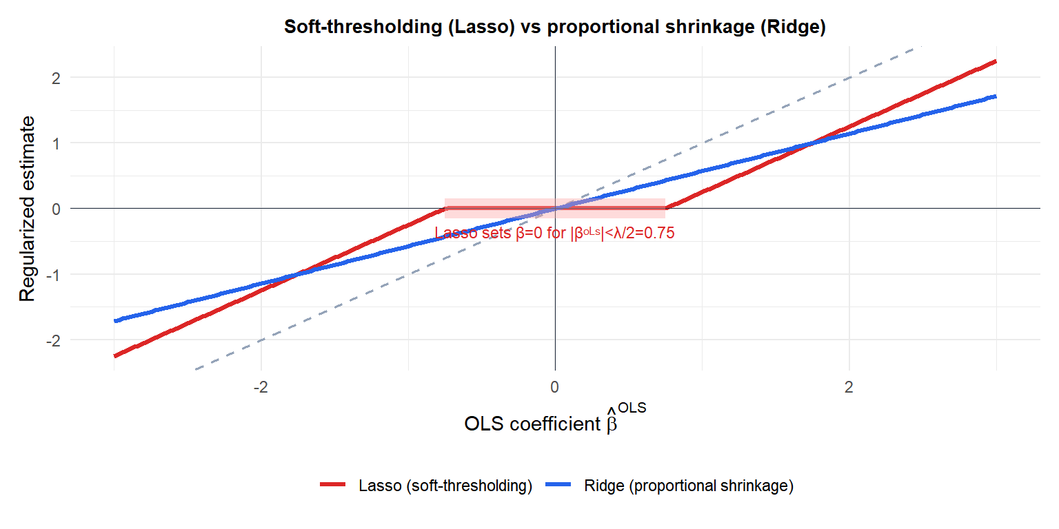
The red zone shows where Lasso sets the coefficient to exactly zero. Ridge (blue) always produces a nonzero estimate, just scaled down. The dashed line is the identity (OLS).
Coordinate descent algorithm
The standard algorithm for fitting Lasso is coordinate descent: cycle through the predictors one at a time, minimizing the objective with respect to \(\beta_j\) while holding all others fixed.
For predictor \(j\), the partial residual is \(\mathbf{r}_j = \mathbf{y} - \sum_{k \neq j} \hat{\beta}_k \mathbf{x}_k\). The update is:
\[\hat{\beta}_j \leftarrow \frac{1}{n}\text{ST}\!\left(\mathbf{x}_j^T \mathbf{r}_j / n,\; \lambda/2\right)\]
where \(\text{ST}\) is the soft-thresholding operator. This is fast and converges to the global minimum because the Lasso objective is convex.
The full Lasso path (solutions for all \(\lambda\)) is computed efficiently by LARS (Least Angle Regression): as \(\lambda\) decreases from \(\infty\) to 0, variables enter the model one at a time. This gives the entire path at roughly the cost of a single OLS fit.
Variable selection in practice
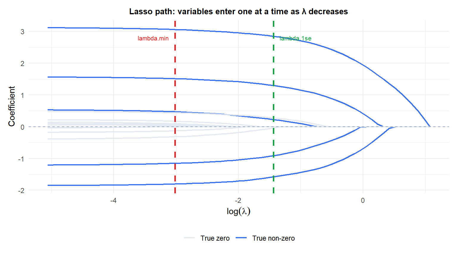
The five true non-zero predictors (blue) enter the model first as \(\lambda\) decreases. The ten true zeros (grey) remain at zero until very small \(\lambda\). The CV-selected \(\lambda\) correctly identifies approximately the right sparsity.
Limitations of Lasso
Correlated predictors: arbitrary selection
When two predictors are highly correlated and both are relevant, Lasso tends to select one arbitrarily and set the other to zero. The selected predictor depends on random variation in the data. This makes Lasso unstable for feature selection when predictors are correlated: run Lasso on two similar datasets and you may get different selected subsets.
Ridge handles correlated predictors better by shrinking both coefficients to similar values. ElasticNet combines both penalties and selects groups of correlated predictors together.
When \(p > n\): Lasso selects at most \(n\) variables
When there are more predictors than observations, Lasso can select at most \(n\) variables (the rank of \(\mathbf{X}\)). If the true model has more than \(n\) relevant predictors, Lasso will miss some. ElasticNet does not have this restriction.
⚠️ Lasso selection is not stable: use with caution for inference
Lasso variable selection is a prediction tool, not a formal statistical test. The selected set of variables can change substantially with small perturbations to the data (bootstrap the variable selection to see how stable it is). Using “Lasso selected these variables” as evidence that they are the true causal predictors is problematic.
For stable variable selection with valid p-values, consider: stability selection, post-selection inference methods (selective inference), or cross-validation on the full variable selection procedure.
💡 Lasso in R
library(glmnet)

# Fit Lasso (alpha=1)
fit_lasso <- glmnet(X, y, alpha=1)
plot(fit_lasso, xvar="lambda", label=TRUE)

# Select lambda by CV
cv_lasso <- cv.glmnet(X, y, alpha=1, nfolds=10)
plot(cv_lasso)

# Selected variables at lambda.1se (sparser, more conservative)
coef_selected <- coef(cv_lasso, s="lambda.1se")
selected_vars  <- rownames(coef_selected)[coef_selected[,1] != 0]

# Bootstrap stability of variable selection
library(dplyr)
B <- 200
selected_counts <- table(unlist(lapply(1:B, function(b) {
  idx <- sample(nrow(X), replace=TRUE)
  cv_b <- cv.glmnet(X[idx,], y[idx], alpha=1)
  cf   <- coef(cv_b, s="lambda.1se")
  rownames(cf)[cf[,1] != 0]
})))
# Variables selected in > 80% of bootstrap samples are stable
