K-nearest neighbors (KNN)
K-nearest neighbors (KNN) is the simplest classification algorithm: to classify a new point, find the \(k\) closest training points and take a majority vote. No training phase, no parameters to estimate, no distributional assumptions. The entire model is the training data itself. Its simplicity makes it an excellent baseline and a useful lens for understanding the bias-variance tradeoff.
The algorithm
Classification: given a new point \(\mathbf{x}\), find the \(k\) training points closest to \(\mathbf{x}\) under some distance metric. Assign the class that appears most frequently among those \(k\) neighbors.
Regression: same neighborhood search, but predict the average (or weighted average) of the response values of the \(k\) neighbors.
Formal prediction rule for classification:
\[\hat{y} = \arg\max_{c} \sum_{i \in \mathcal{N}_k(\mathbf{x})} \mathbf{1}[y_i = c]\]
where \(\mathcal{N}_k(\mathbf{x})\) is the set of \(k\) nearest neighbors of \(\mathbf{x}\).
KNN is a lazy learner: it does no work at training time and defers all computation to prediction time. This makes training instant but prediction slow for large datasets.
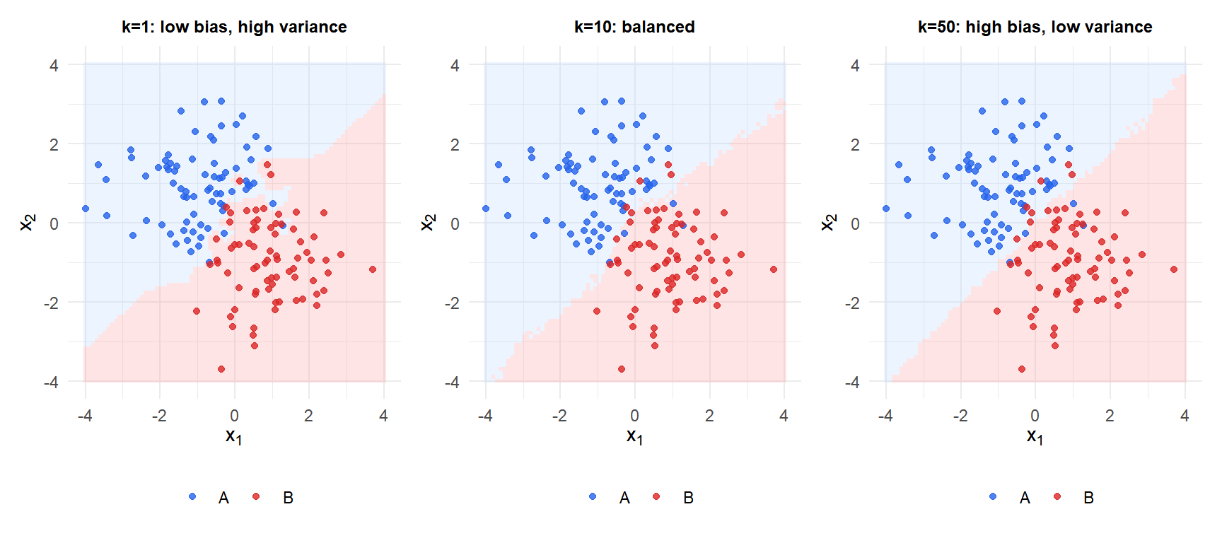
The effect of k: bias-variance tradeoff
\(k\) is the only hyperparameter and it directly controls model complexity:
- Small \(k\) (e.g., \(k=1\)): each point is its own neighborhood. The decision boundary is highly irregular, adapting to every training point including noise. Low bias, high variance. With \(k=1\), training error is always zero.
- Large \(k\) (e.g., \(k=n\)): every point is classified as the overall majority class regardless of location. Very smooth boundary. High bias, low variance.
The optimal \(k\) is selected by cross-validation. A common starting point: \(k = \sqrt{n}\), though CV almost always finds a better value.
Distance metrics
KNN is entirely defined by the chosen distance metric. The result changes substantially with the metric.
Minkowski distance (general family):
\[d_p(\mathbf{x}, \mathbf{x}') = \left(\sum_{j=1}^p |x_j - x_j'|^p\right)^{1/p}\]
Special cases:
- \(p=1\): Manhattan distance (L1). Sum of absolute differences. Less sensitive to outliers in individual features.
- \(p=2\): Euclidean distance (L2). Most common default. Sensitive to scale.
- \(p \to \infty\): Chebyshev distance. Maximum absolute difference across dimensions.
For categorical features: Hamming distance (proportion of mismatched attributes). For mixed types: Gower distance.
⚠️ Always standardize features before applying KNN
Euclidean distance is dominated by features with large scales. If one feature ranges from 0 to 10{,}000 and another from 0 to 1, the first feature will control the distance calculation entirely and the second will be effectively ignored.
Always standardize features to zero mean and unit variance (or scale to [0,1]) before fitting KNN. This is not optional: without standardization, the choice of units determines the model.
The curse of dimensionality
KNN relies on the assumption that nearby points in feature space are similar. In high dimensions, this assumption breaks down severely.
Consider a hypercube \([0,1]^d\) with \(n\) uniformly distributed training points. To capture a fraction \(r\) of the data volume for a neighborhood, the expected side length of the hypercube neighborhood is \(r^{1/d}\). For \(r=0.01\) (1% of the data):
- \(d=2\): side length \(\approx 0.1\) (10% of the range per dimension)
- \(d=10\): side length \(\approx 0.63\) (63% of the range per dimension)
- \(d=100\): side length \(\approx 0.955\) (95.5% of the range per dimension)
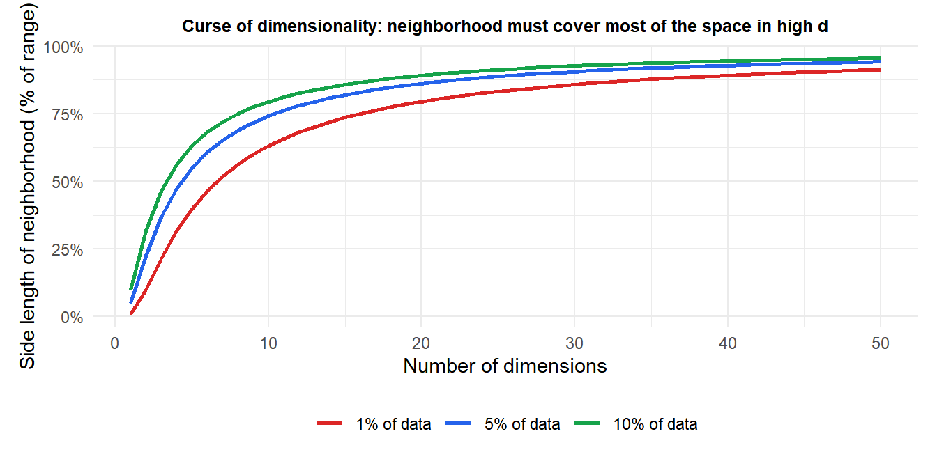
In high dimensions, the nearest neighbors are barely closer than the farthest points. All points become approximately equidistant, and the concept of “nearness” loses meaning. KNN performance degrades rapidly above \(d \approx 10\)-20 features.
Weighted KNN
Standard KNN gives equal weight to all \(k\) neighbors. Weighted KNN gives more weight to closer neighbors:
\[\hat{y} = \arg\max_c \sum_{i \in \mathcal{N}_k(\mathbf{x})} w_i \cdot \mathbf{1}[y_i = c], \qquad w_i = \frac{1}{d(\mathbf{x}, \mathbf{x}_i)^2}\]
Inverse-distance weighting reduces the influence of the farthest neighbors in the neighborhood, often improving accuracy without changing \(k\).
Computational complexity and speed-up structures
Naive KNN has prediction complexity \(O(nd)\) per query: compute distance to all \(n\) training points in \(d\) dimensions. For large \(n\) or \(d\) this is slow.
Two data structures reduce this cost:
kd-tree: a binary tree that partitions the feature space recursively by splitting along one dimension at a time. For \(d \leq 20\) and large \(n\), query time drops to \(O(d\log n)\) average. Performance degrades in high dimensions.
Ball tree: partitions points into nested hyperspheres. More effective than kd-trees in moderate to high dimensions.
Both structures are built at training time (\(O(nd\log n)\)) and queried at prediction time. The FNN and class packages in R, and sklearn in Python, use these structures automatically.
💡 KNN in R
library(class)

# Standardize features
X_train_s <- scale(X_train)
X_test_s  <- scale(X_test,
                   center=attr(X_train_s,"scaled:center"),
                   scale =attr(X_train_s,"scaled:scale"))

# Classify with k=10
pred <- knn(train=X_train_s, test=X_test_s, cl=y_train, k=10)

# Select k by cross-validation
library(caret)
ctrl <- trainControl(method="cv", number=10)
fit  <- train(y ~ ., data=df, method="knn",
              trControl=ctrl,
              tuneGrid=data.frame(k=c(1,3,5,10,20,50)))
fit$bestTune

# Weighted KNN
library(kknn)
fit_w <- kknn(y ~ ., train=df_train, test=df_test, k=10,
              kernel="triangular")  # distance-weighted
