Hierarchical clustering
Hierarchical clustering builds a nested sequence of clusters without requiring the number of clusters \(K\) in advance. The result is a dendrogram: a tree where each leaf is an observation and each internal node records when two clusters merged. Cutting the tree at any height yields a flat clustering. The linkage method, which defines the distance between clusters, has a larger impact on the result than almost any other choice.
Agglomerative clustering
The most common variant is agglomerative (bottom-up):
- Start with \(n\) clusters, one per observation.
- Compute the \(n \times n\) dissimilarity matrix.
- Merge the two closest clusters into one.
- Update the dissimilarity matrix (how the new cluster’s distances are computed depends on the linkage).
- Repeat steps 3-4 until one cluster remains.
The merge history is stored in the dendrogram. The height at which two observations (or clusters) merge reflects how dissimilar they are: low merges = similar, high merges = dissimilar.
Divisive clustering works top-down: start with all observations in one cluster and recursively split. Computationally heavier and less commonly used.
Linkage methods
The linkage method defines the distance \(d(A, B)\) between two clusters \(A\) and \(B\) based on their constituent point distances:
| Linkage | Formula | Shape of clusters |
|---|---|---|
| Single | \(\min_{a \in A, b \in B} d(a,b)\) | Elongated, chaining |
| Complete | \(\max_{a \in A, b \in B} d(a,b)\) | Compact, roughly spherical |
| Average (UPGMA) | \(\frac{1}{|A||B|}\sum_{a,b} d(a,b)\) | Between single and complete |
| Centroid | \(d(\bar{a}, \bar{b})\) | Can invert (non-monotone) |
| Ward | Increase in total WCSS from merging \(A\) and \(B\) | Compact, equal-sized |
Ward’s linkage merges the pair of clusters that minimizes the increase in total within-cluster sum of squares. It tends to produce compact, roughly equal-sized clusters and is the default choice for most applications with continuous data.
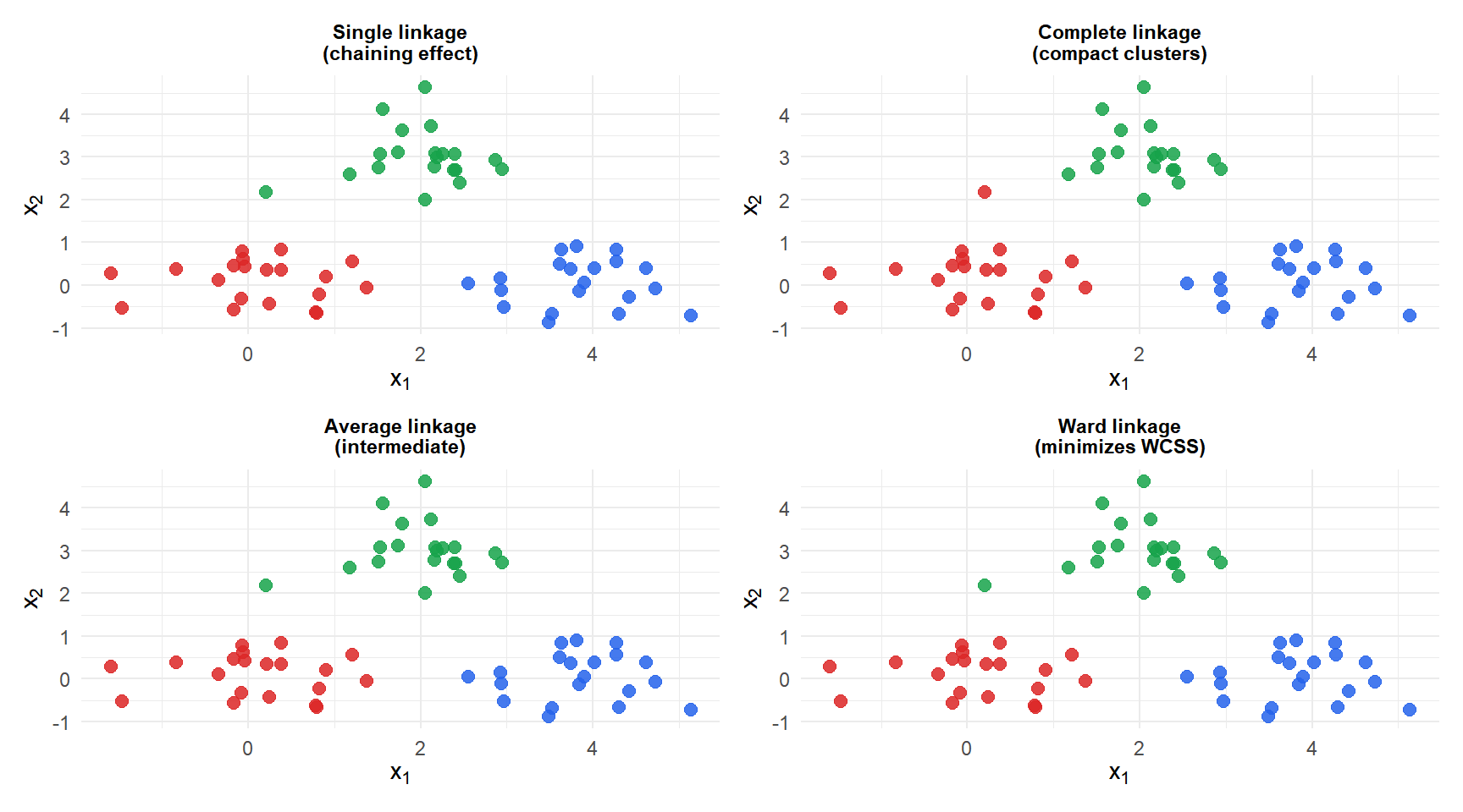
Single linkage (top-left) chains clusters together, often producing elongated groups. Complete linkage produces compact clusters. Average linkage is intermediate. Ward (bottom-right) produces the most balanced, compact clusters and usually matches the visual grouping most closely.
Reading the dendrogram
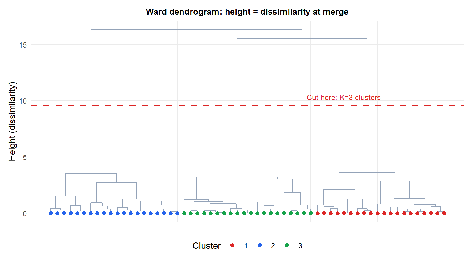
The dashed red line cuts the tree at a chosen height. Every vertical line it crosses becomes a cluster. Here cutting at this height gives three clusters (matching the true structure). The height axis represents dissimilarity: merges low in the tree join similar observations; merges near the top join very different groups.
Choosing the cut height: look for the largest gap between consecutive merge heights. A big gap means the two levels of the hierarchy are very different: the cut just below the gap is a natural number of clusters.
Distance matrices and non-Euclidean data
Hierarchical clustering works with any dissimilarity matrix, not just Euclidean distance. This makes it applicable to data types where Euclidean distance is meaningless:
- Text: cosine distance or edit distance between documents.
- Categorical data: Gower distance (handles mixed types).
- Sequences: edit distance (Levenshtein) for DNA or protein sequences.
- Time series: dynamic time warping distance.
- Correlation-based: \(1 - r_{ij}\) where \(r_{ij}\) is the Pearson correlation. Widely used in genomics to cluster genes with similar expression profiles.
K-means requires computing means (centroids) and thus only works with Euclidean distance on continuous data. Hierarchical clustering works with any custom dissimilarity.
Hierarchical clustering vs K-means
| Hierarchical | K-means | |
|---|---|---|
| Requires K upfront | No | Yes |
| Result | Full hierarchy (dendrogram) | Flat partition |
| Deterministic | Yes | No (random init) |
| Scalability | \(O(n^2)\) to \(O(n^3)\) | \(O(nKI)\), fast |
| Non-Euclidean data | Yes (any dissimilarity) | No |
| Cluster shapes | Flexible (depends on linkage) | Spherical only |
| Sensitivity to outliers | High (especially single linkage) | Moderate |
Use hierarchical clustering when: you do not know \(K\), you want to explore the hierarchy, the data is not Euclidean, or \(n\) is small enough for the quadratic complexity (\(n < 10{,}000\) typically).
Use K-means when: \(K\) is known or can be estimated, the data is large, and clusters are roughly spherical.
⚠️ Single linkage is almost never the right choice
Single linkage is notorious for the chaining effect: a single bridge point connecting two clusters causes them to merge prematurely, creating long, string-like clusters that do not reflect the true structure. Unless the true clusters are genuinely filamentous (rare), always start with Ward, complete, or average linkage and only consider single linkage if there is a specific reason.
💡 Hierarchical clustering in R
# Compute dissimilarity matrix
d <- dist(X, method="euclidean")   # or "manhattan", "maximum"

# Fit hierarchical clustering
hc <- hclust(d, method="ward.D2")  # or "complete", "average", "single"

# Visualize dendrogram
plot(hc, labels=FALSE, hang=-1)
rect.hclust(hc, k=3, border="red")  # draw K clusters

# Cut to K clusters
clusters <- cutree(hc, k=3)
# Or cut at a specific height
clusters <- cutree(hc, h=5)

# Non-Euclidean: Gower distance for mixed data
library(cluster)
d_gower <- daisy(df_mixed, metric="gower")
hc_g    <- hclust(d_gower, method="ward.D2")

# Pretty dendrograms
library(ggdendro)
ggdendrogram(hc, rotate=FALSE, labels=FALSE)
