ElasticNet regression
ElasticNet combines the \(L_1\) penalty of Lasso with the \(L_2\) penalty of Ridge. It inherits Lasso’s ability to set coefficients exactly to zero (variable selection) while fixing Lasso’s two main weaknesses: instability with correlated predictors and the \(p > n\) restriction. A single mixing parameter \(\alpha\) controls the blend between the two penalties.
Objective function
\[\hat{\boldsymbol{\beta}}^{EN} = \arg\min_{\boldsymbol{\beta}} \|\mathbf{y} - \mathbf{X}\boldsymbol{\beta}\|_2^2 + \lambda\left[\alpha\|\boldsymbol{\beta}\|_1 + \frac{1-\alpha}{2}\|\boldsymbol{\beta}\|_2^2\right]\]
Two hyperparameters:
- \(\lambda \geq 0\): overall regularization strength. Larger \(\lambda\) shrinks more.
- \(\alpha \in [0,1]\): mixing parameter.
- \(\alpha = 1\): pure Lasso.
- \(\alpha = 0\): pure Ridge.
- \(\alpha \in (0,1)\): ElasticNet blend.
The \(1/2\) factor in the \(L_2\) term is a convention that simplifies derivatives; the key point is that \(\alpha\) controls the relative weight between the two penalties.
Why ElasticNet exists: the two problems with Lasso
Problem 1: correlated predictors
When two predictors \(x_j\) and \(x_k\) are highly correlated and both relevant, Lasso picks one arbitrarily and sets the other to zero. The selection depends on random variation in the data: run Lasso twice on slightly different samples and you may get different selected subsets.
The \(L_2\) component of ElasticNet introduces a grouping effect: when predictors are correlated, ElasticNet tends to include or exclude them together, assigning similar coefficients to predictors that provide similar information. The bound on the difference between correlated coefficients is:
\[|\hat{\beta}_j^{EN} - \hat{\beta}_k^{EN}| \leq \frac{1}{\lambda(1-\alpha)}\sqrt{2(1-r_{jk})}\]
where \(r_{jk}\) is the correlation between \(x_j\) and \(x_k\). As \(r_{jk} \to 1\), the two coefficients converge to the same value.
Problem 2: \(p > n\) situations
Lasso can select at most \(n\) variables when \(p > n\) (the rank of \(\mathbf{X}\) limits the number of nonzero coefficients). ElasticNet has no such restriction: the \(L_2\) component stabilizes the optimization and allows more than \(n\) variables to be selected simultaneously.
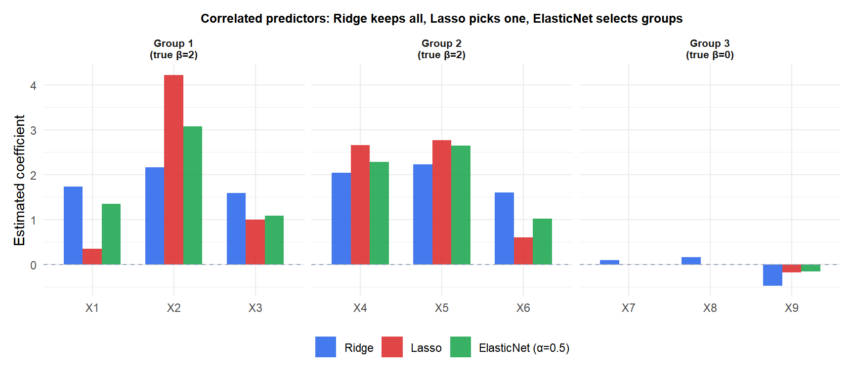
With three groups of correlated predictors: Ridge (blue) keeps all with similar coefficients; Lasso (red) picks one per group arbitrarily; ElasticNet (green) selects the group together, assigning similar nonzero coefficients to correlated predictors and zeroing the irrelevant group.
Effect of the mixing parameter \(\alpha\)
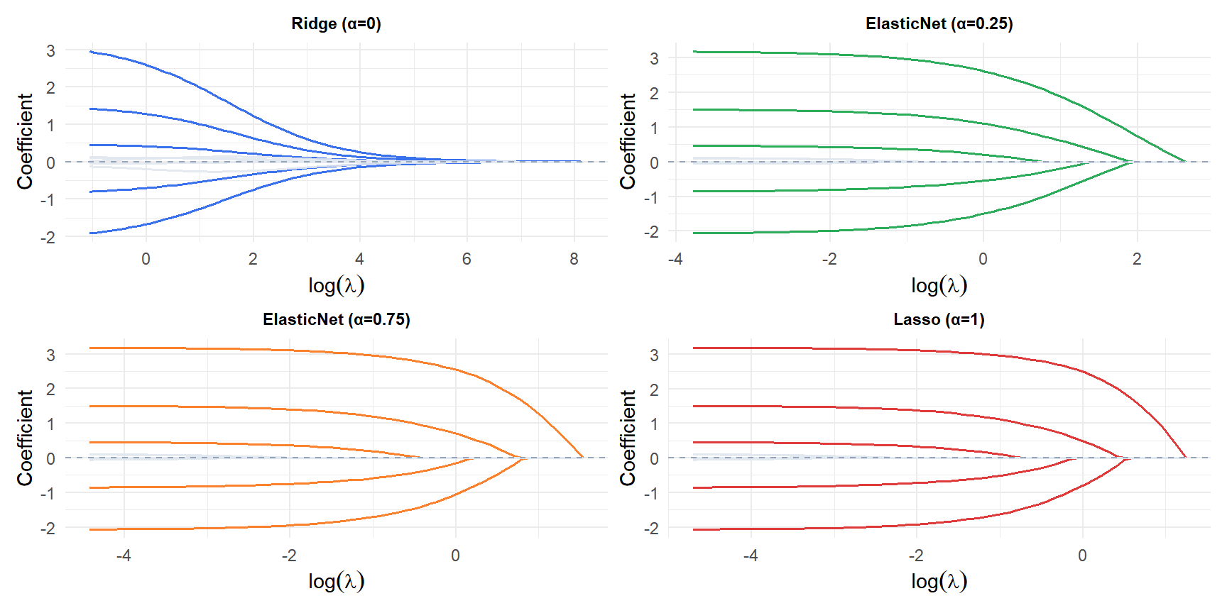
As \(\alpha\) increases from 0 (Ridge) to 1 (Lasso), the coefficient paths transition from smooth shrinkage to hard thresholding. At \(\alpha=0.25\) and \(\alpha=0.75\) the behavior is intermediate: some coefficients reach zero but less abruptly than pure Lasso.
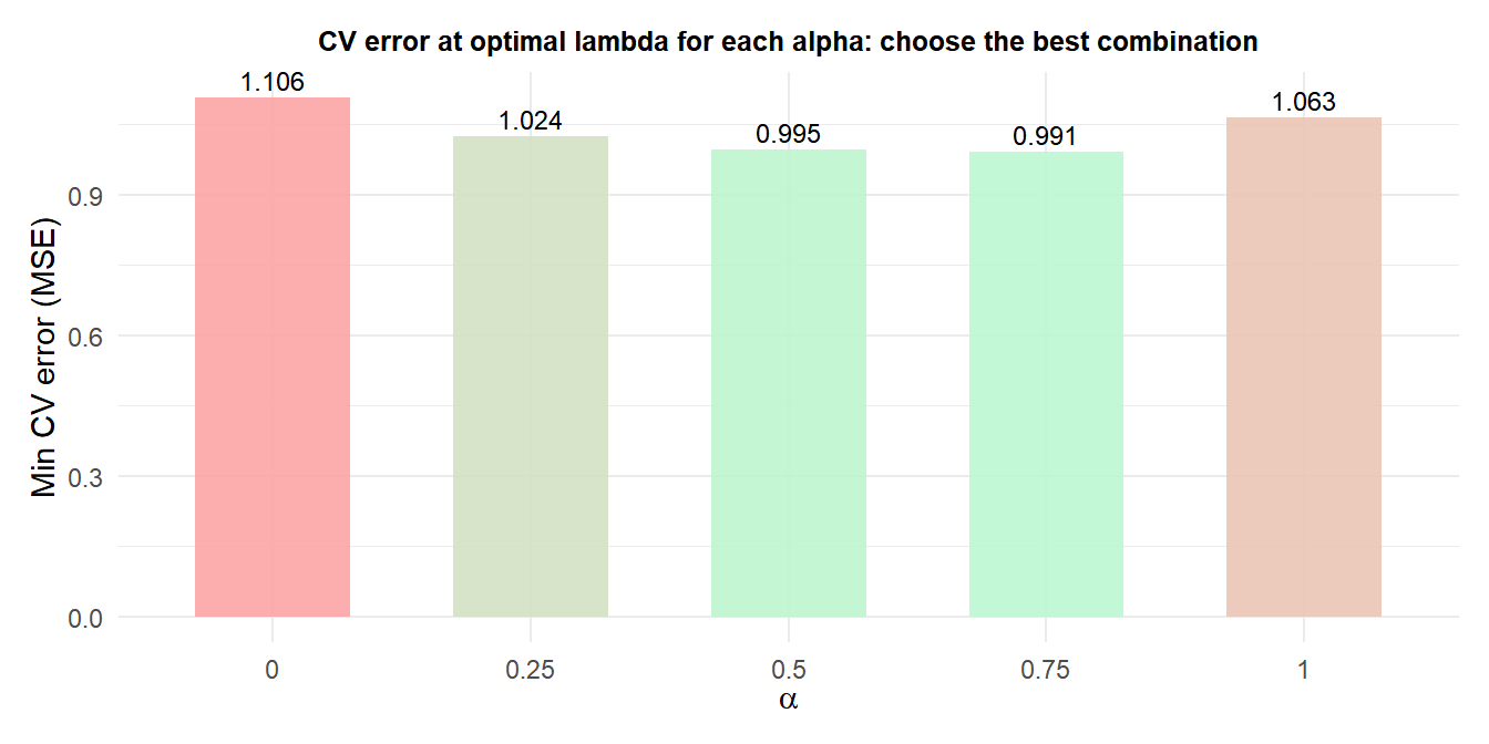
Selecting \(\alpha\) and \(\lambda\)
Both \(\alpha\) and \(\lambda\) must be selected. The standard approach is a nested grid search with cross-validation:
- Define a grid of \(\alpha\) values (e.g., 0, 0.1, 0.25, 0.5, 0.75, 0.9, 1).
- For each \(\alpha\), run
cv.glmnetto find the optimal \(\lambda\). - Select the \((\alpha, \lambda)\) pair with the lowest CV error.
Ridge, Lasso or ElasticNet?
| Situation | Recommended method |
|---|---|
| All predictors relevant, dense signal | Ridge |
| Sparse signal, predictors independent | Lasso |
| Sparse signal, correlated predictors | ElasticNet |
| \(p \gg n\), many relevant predictors | ElasticNet |
| Variable selection is the goal | Lasso or ElasticNet |
| Prediction only, no interpretability needed | Any; tune \(\alpha\) by CV |
In practice, ElasticNet with CV-selected \(\alpha\) rarely performs worse than either Ridge or Lasso, because it includes both as special cases. The cost is one extra hyperparameter.
⚠️ Double penalization changes the effective lambda scale
The ElasticNet penalty is \(\lambda[\alpha|\beta_j| + (1-\alpha)\beta_j^2/2]\). The \(L_2\) term shrinks coefficients even when \(\alpha\) is close to 1, which means the effective regularization is stronger than pure Lasso at the same \(\lambda\). When comparing models across different \(\alpha\) values, always compare at the CV-optimal \(\lambda\) for each \(\alpha\), not at the same nominal \(\lambda\).
Also: standardize predictors before fitting. glmnet does this by default.
💡 ElasticNet in R
library(glmnet)

# Single alpha: ElasticNet with alpha=0.5
fit_en <- glmnet(X, y, alpha=0.5)
cv_en  <- cv.glmnet(X, y, alpha=0.5, nfolds=10)
coef(cv_en, s="lambda.min")

# Grid search over alpha and lambda
alphas <- c(0, 0.25, 0.5, 0.75, 1)
cv_list <- lapply(alphas, function(a)
  cv.glmnet(X, y, alpha=a, nfolds=10))

# Best combination
best_cvm <- sapply(cv_list, function(cv) min(cv$cvm))
best_alpha  <- alphas[which.min(best_cvm)]
best_lambda <- cv_list[[which.min(best_cvm)]]$lambda.min

# Fit final model
fit_final <- glmnet(X, y, alpha=best_alpha, lambda=best_lambda)
coef(fit_final)
