Discriminant analysis
Linear Discriminant Analysis (LDA) and Quadratic Discriminant Analysis (QDA) classify observations by modeling the class-conditional distribution of the features as multivariate Gaussians and applying Bayes’ theorem. LDA assumes all classes share the same covariance matrix, giving linear decision boundaries; QDA allows each class its own covariance, giving quadratic boundaries.
The generative model
Both LDA and QDA model each class \(k\) as a multivariate Gaussian:
\[P(\mathbf{x} \mid C=k) = \frac{1}{(2\pi)^{p/2}|\boldsymbol{\Sigma}_k|^{1/2}} \exp\!\left(-\frac{1}{2}(\mathbf{x}-\boldsymbol{\mu}_k)^T\boldsymbol{\Sigma}_k^{-1}(\mathbf{x}-\boldsymbol{\mu}_k)\right)\]
Applying Bayes’ theorem, the posterior probability of class \(k\) is:
\[P(C=k \mid \mathbf{x}) \propto \pi_k \cdot P(\mathbf{x} \mid C=k)\]
where \(\pi_k = P(C=k)\) is the prior probability of class \(k\), estimated as the class proportion in the training data.
Linear Discriminant Analysis (LDA)
LDA adds the constraint \(\boldsymbol{\Sigma}_1 = \boldsymbol{\Sigma}_2 = \cdots = \boldsymbol{\Sigma}_K = \boldsymbol{\Sigma}\) (equal covariance matrices). Under this constraint, the log-posterior ratio between two classes simplifies to a linear function of \(\mathbf{x}\):
\[\delta_k(\mathbf{x}) = \mathbf{x}^T\boldsymbol{\Sigma}^{-1}\boldsymbol{\mu}_k - \frac{1}{2}\boldsymbol{\mu}_k^T\boldsymbol{\Sigma}^{-1}\boldsymbol{\mu}_k + \log\pi_k\]
\[\hat{c} = \arg\max_k \delta_k(\mathbf{x})\]
The quadratic term \(\mathbf{x}^T\boldsymbol{\Sigma}^{-1}\mathbf{x}\) is the same for all classes and cancels in the comparison, leaving a linear function of \(\mathbf{x}\). The decision boundary between classes \(j\) and \(k\) is the set of points where \(\delta_j(\mathbf{x}) = \delta_k(\mathbf{x})\): a hyperplane.
Parameter estimation: \(\hat{\boldsymbol{\mu}}_k\) = class sample means; \(\hat{\boldsymbol{\Sigma}}\) = pooled within-class sample covariance.
Fisher’s criterion: maximizing class separation
An equivalent way to derive LDA: find the projection direction \(\mathbf{w}\) that maximizes the ratio of between-class variance to within-class variance after projecting the data onto \(\mathbf{w}\):
\[\mathbf{w}^* = \arg\max_{\mathbf{w}} \frac{\mathbf{w}^T \mathbf{S}_B \mathbf{w}}{\mathbf{w}^T \mathbf{S}_W \mathbf{w}}\]
where \(\mathbf{S}_B = \sum_k n_k(\boldsymbol{\mu}_k - \boldsymbol{\mu})(\boldsymbol{\mu}_k - \boldsymbol{\mu})^T\) is the between-class scatter matrix and \(\mathbf{S}_W = \sum_k \sum_{i \in C_k}(\mathbf{x}_i - \boldsymbol{\mu}_k)(\mathbf{x}_i - \boldsymbol{\mu}_k)^T\) is the within-class scatter matrix.
The solution is \(\mathbf{w}^* = \mathbf{S}_W^{-1}(\boldsymbol{\mu}_1 - \boldsymbol{\mu}_2)\) for two classes. For \(K\) classes, the first \(K-1\) discriminant directions are the eigenvectors of \(\mathbf{S}_W^{-1}\mathbf{S}_B\) corresponding to the largest eigenvalues.
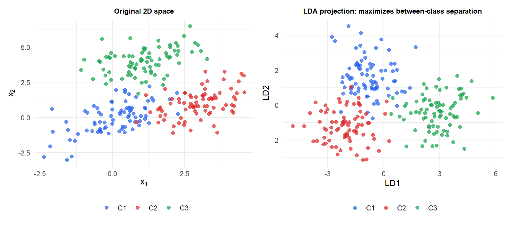
This is the dimensionality reduction perspective of LDA: project onto the \(K-1\) directions that best separate the classes, then classify in the reduced space.
Quadratic Discriminant Analysis (QDA)
QDA relaxes the equal covariance assumption. Each class has its own covariance \(\boldsymbol{\Sigma}_k\), and the log-posterior does not simplify to a linear function:
\[\delta_k(\mathbf{x}) = -\frac{1}{2}\log|\boldsymbol{\Sigma}_k| - \frac{1}{2}(\mathbf{x}-\boldsymbol{\mu}_k)^T\boldsymbol{\Sigma}_k^{-1}(\mathbf{x}-\boldsymbol{\mu}_k) + \log\pi_k\]
The term \((\mathbf{x}-\boldsymbol{\mu}_k)^T\boldsymbol{\Sigma}_k^{-1}(\mathbf{x}-\boldsymbol{\mu}_k)\) is the squared Mahalanobis distance from \(\mathbf{x}\) to class \(k\)’s centroid, weighted by the class covariance. The decision boundary between classes \(j\) and \(k\) is a quadratic surface (ellipse, parabola, or hyperbola in 2D).
QDA estimates \(p(p+1)/2\) parameters per class for the covariance matrix, versus LDA’s single pooled \(\boldsymbol{\Sigma}\). With \(K\) classes: QDA has \(K \cdot p(p+1)/2\) covariance parameters vs LDA’s \(p(p+1)/2\).
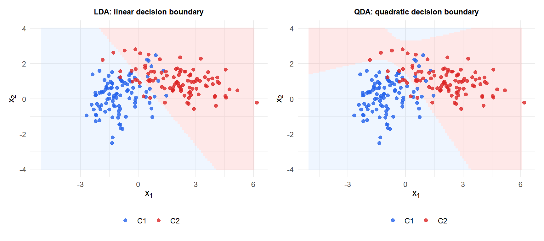
With unequal covariances (C2 has higher variance and negative correlation), LDA forces a straight boundary that misclassifies points in the tails. QDA curves the boundary to better match the true class structure.
LDA as dimensionality reduction
For \(K\) classes in \(p\) dimensions, LDA projects the data onto at most \(K-1\) discriminant directions before classifying. This makes LDA a useful preprocessing step:
- Reduces \(p\) dimensions to \(K-1\) for visualization or as input to another classifier.
- Unlike PCA (which maximizes total variance), LDA maximizes class separation in the reduced space.
- For \(K=2\): a single discriminant axis separates the two classes. Plot the 1D projection to visualize separability.
- For \(K=3\): two discriminant axes give a 2D plot that shows the class structure.
⚠️ LDA fails when the equal covariance assumption is strongly violated
When classes have very different covariances, LDA’s linear boundary is misspecified and accuracy degrades. Signs of violation: different spread or shape of point clouds per class, the covariance matrices look very different numerically.
Test with Box’s M test (biotools::boxM()) for formal equality of covariance matrices. If rejected, use QDA. Note that QDA needs more data: each class needs at least \(p+1\) observations to estimate its covariance matrix, and ideally many more for stable estimates.
LDA vs QDA vs logistic regression
| LDA | QDA | Logistic regression | |
|---|---|---|---|
| Decision boundary | Linear | Quadratic | Linear (standard) |
| Assumption | Gaussian, equal \(\boldsymbol{\Sigma}\) | Gaussian, different \(\boldsymbol{\Sigma}\) | None on \(P(\mathbf{x})\) |
| Parameters | Few | More (\(K\) covariances) | \(p+1\) |
| Stable with small \(n\) | Yes | Needs more data | Yes |
| Also does dim. reduction | Yes (\(K-1\) axes) | No | No |
| Sensitive to outliers | Moderate | More | Less |
LDA tends to outperform logistic regression when the Gaussian assumption is approximately correct and \(n\) is small. Logistic regression is more robust to non-Gaussian features and outliers. QDA wins when classes genuinely have different covariance structures and enough data is available to estimate them reliably.
💡 Discriminant analysis in R
library(MASS)

# LDA
fit_lda <- lda(y ~ ., data=df_train)
predict(fit_lda, newdata=df_test)$class      # predicted classes
predict(fit_lda, newdata=df_test)$posterior  # posterior probabilities
predict(fit_lda, newdata=df_test)$x          # LD scores (for plotting)

# QDA
fit_qda <- qda(y ~ ., data=df_train)
predict(fit_qda, newdata=df_test)$class

# Test equal covariances (Box's M test)
library(biotools)
boxM(df_train[,-1], df_train$y)

# Regularized LDA (for p close to n)
library(klaR)
fit_rda <- rda(y ~ ., data=df_train, gamma=0.05, lambda=0.2)
