Cross-validation
Cross-validation estimates how well a model will perform on new, unseen data by repeatedly partitioning the available data into training and validation sets. It is the standard tool for model evaluation, hyperparameter selection, and comparing competing models. Using it incorrectly produces optimistic estimates that fail to generalize.
Why a single train/test split is not enough
Splitting the data once into training and test sets is simple but noisy: the estimated performance depends heavily on which observations end up in each set. With \(n=200\) and an 80/20 split, the test set has only 40 observations: the estimated error has high variance across different random splits.
Cross-validation addresses this by using multiple splits and averaging the results. The estimate is more stable, and we get a measure of its uncertainty (standard deviation across folds).
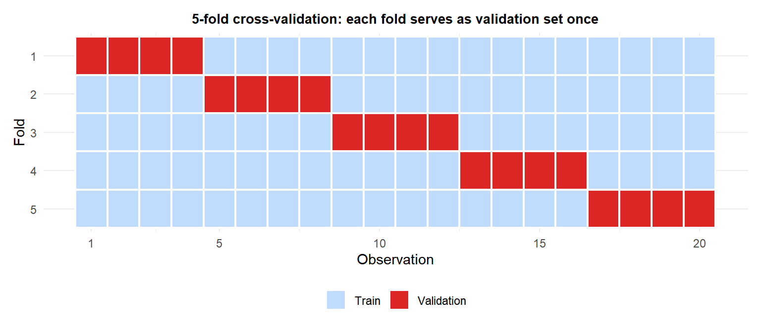
K-fold cross-validation
Partition the data randomly into \(k\) folds of approximately equal size. For each fold \(i = 1, \ldots, k\):
- Train the model on the \(k-1\) other folds.
- Evaluate on fold \(i\), recording the metric (e.g., MSE, accuracy).
The CV estimate is the mean across all \(k\) folds:
\[\widehat{\text{CV}}_k = \frac{1}{k}\sum_{i=1}^k \text{error}_i\]
\[\widehat{\text{SE}} = \sqrt{\frac{1}{k(k-1)}\sum_{i=1}^k(\text{error}_i - \widehat{\text{CV}}_k)^2}\]
The standard error \(\widehat{\text{SE}}\) quantifies the uncertainty of the CV estimate. The one-standard-error rule: when comparing models, choose the simplest model whose CV error is within one SE of the minimum. This prefers parsimony without sacrificing much accuracy.
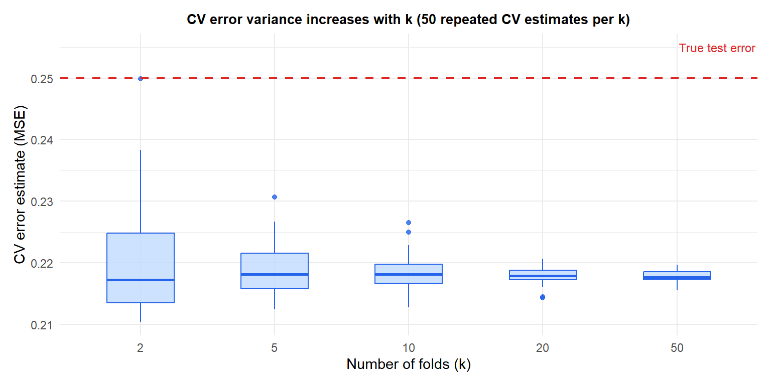
Choosing k: the bias-variance tradeoff
The choice of \(k\) controls a bias-variance tradeoff in the CV estimate itself:
- Large \(k\) (e.g., LOOCV): training sets are close to size \(n\) (low bias). But the \(k\) validation sets are almost identical (the models trained on them are highly correlated), so the variance of the CV estimate is high.
- Small \(k\) (e.g., \(k=2\)): training sets have only \(n/2\) observations (high bias: the model is weaker than it would be on the full data). Low variance.
- \(k=5\) or \(k=10\): empirically shown to give good bias-variance balance. The standard choice.
LOOCV (\(k=n\)) has one special property: for linear models, there is a shortcut formula that computes LOOCV without refitting \(n\) times:
\[\text{LOOCV} = \frac{1}{n}\sum_{i=1}^n \left(\frac{y_i - \hat{y}_i}{1 - h_{ii}}\right)^2\]
where \(h_{ii}\) is the leverage of observation \(i\). This makes LOOCV practical for linear models but it still has high variance as an estimator.
Variants of cross-validation
Stratified k-fold
For classification with imbalanced classes, ensure each fold has the same class proportions as the full dataset. Without stratification, a fold may contain very few minority class examples, making the error estimate noisy and unrepresentative. Always use stratified CV for classification.
Repeated k-fold
Repeat \(k\)-fold CV \(r\) times with different random partitions. Average over all \(r \times k\) folds. Gives more stable estimates at the cost of \(r\) times more computation. Useful when \(n\) is small.
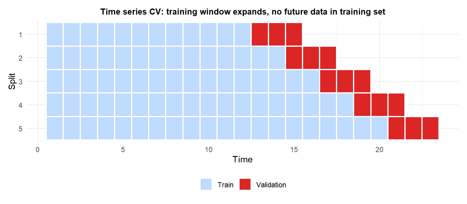
Time series CV (walk-forward validation)
Standard k-fold randomly shuffles the data, creating training folds that contain future observations. For time series this is data leakage: the model “sees the future” during training.
Time series CV uses expanding or sliding windows: train on observations \(1, \ldots, t\) and evaluate on \(t+1, \ldots, t+h\) for increasing values of \(t\).
Nested cross-validation: avoiding data leakage
A common mistake: use CV to select hyperparameters, then report that same CV error as the model’s performance estimate. This is optimistic because the test folds influenced the hyperparameter selection.
Nested CV uses two loops:
- Outer loop: \(k_\text{outer}\) folds for unbiased performance estimation.
- Inner loop: for each outer training set, run \(k_\text{inner}\)-fold CV to select hyperparameters.
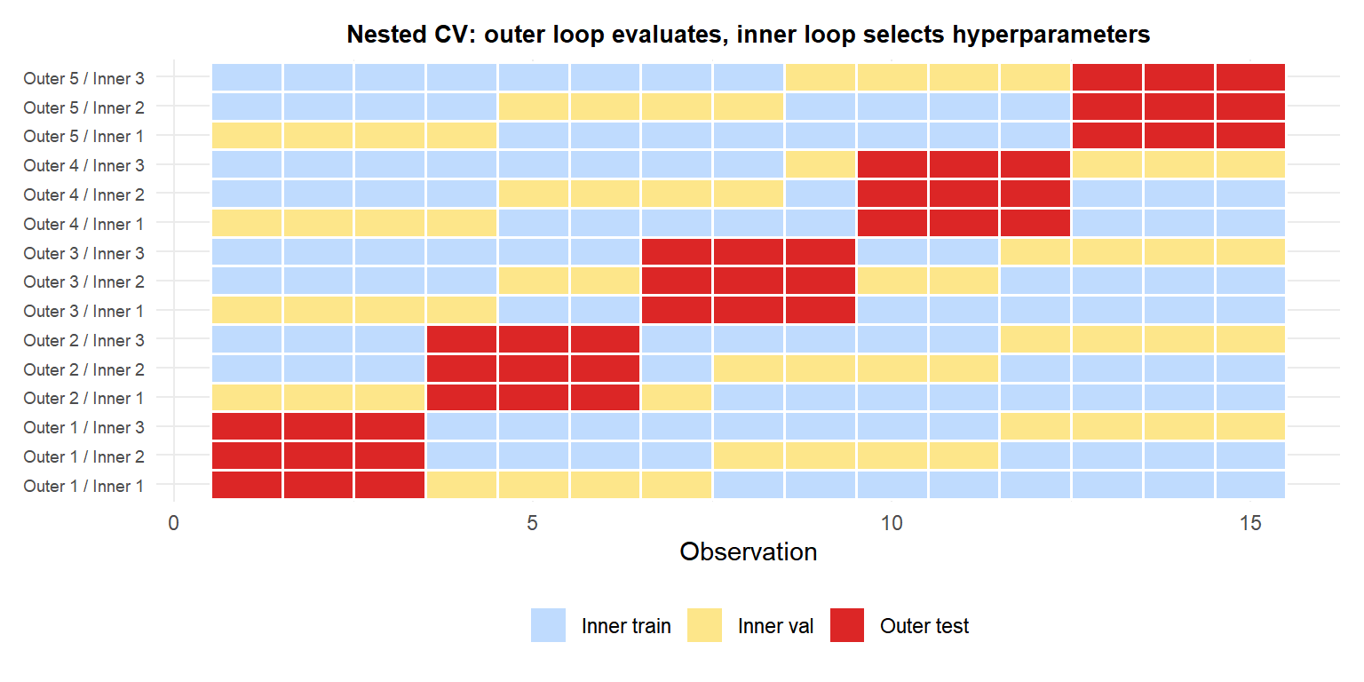
The outer test folds (red) are never seen during hyperparameter selection. The inner validation folds (yellow) are used to select the best hyperparameters for each outer fold’s training set. The outer CV error is an unbiased estimate of the final model’s performance.
⚠️ Using CV error for model selection and reporting is double-dipping
If you use CV to select among 50 models and report the CV error of the winner, the reported error is optimistic: you searched over 50 models and picked the luckiest one. The more models you compare, the larger the optimism.
Correct procedure: use nested CV, or reserve a final holdout test set that is never used for any model selection decision (no hyperparameter tuning, no feature selection, no model comparison). The holdout test set is used exactly once, at the very end, to report the final performance.
💡 Cross-validation in R
library(caret)

# 10-fold CV
ctrl <- trainControl(method="cv", number=10)
fit  <- train(y ~ ., data=df, method="glm", trControl=ctrl)
fit$results   # CV metrics per fold
fit$resample  # individual fold results

# Stratified k-fold for classification
ctrl_strat <- trainControl(method="cv", number=10,
                            classProbs=TRUE, summaryFunction=twoClassSummary)

# Repeated 10-fold
ctrl_rep <- trainControl(method="repeatedcv", number=10, repeats=5)

# Nested CV
library(mlr3)
library(mlr3tuning)
task    <- as_task_classif(df, target="y")
learner <- lrn("classif.ranger", predict_type="prob")
resampling_outer <- rsmp("cv", folds=5)
resampling_inner <- rsmp("cv", folds=3)
measure  <- msr("classif.auc")
tuner    <- tnr("grid_search")
at <- AutoTuner$new(learner, resampling_inner, measure, tuner=tuner,
                    terminator=trm("evals", n_evals=20))
rr <- resample(task, at, resampling_outer)
rr$aggregate(measure)   # unbiased performance estimate
