One-sample z-test for a mean
The one-sample z-test for a mean is used when the population standard deviation \(\sigma\) is known. In practice this is rare: \(\sigma\) is almost never truly known, and the \(t\)-test should be used instead. The z-test remains useful as a pedagogical tool and in a few specific applied contexts.
When to use the z-test vs the t-test
Both tests evaluate \(H_0: \mu = \mu_0\), but they differ in what is assumed about \(\sigma\):
| Z-test | T-test | |
|---|---|---|
| \(\sigma\) | Known | Unknown (estimated by \(S\)) |
| Reference distribution | \(N(0,1)\) | \(t(n-1)\) |
| When to use | \(\sigma\) truly known from prior data or theory | Almost always |
For large \(n\), the \(t\) distribution converges to the standard normal and the two tests give nearly identical results. For small \(n\), the \(t\)-test is more conservative (wider critical region) and correct.
⚠️ Using S in place of σ and calling it a z-test is wrong
A common mistake: compute \(Z = (\bar{X} - \mu_0)/(S/\sqrt{n})\) and compare to \(z_{\alpha/2} = 1.96\). This is incorrect. When \(\sigma\) is replaced by \(S\), the statistic no longer follows a standard normal: it follows a \(t\) distribution. Using \(z\) critical values underestimates the uncertainty and produces anticonservative tests.
The only situations where \(\sigma\) can be considered truly known:
- Historical process control data with very large baseline samples (e.g., a manufacturing process monitored for years).
- Standardized tests where the population SD is established by the testing authority.
- Theoretical distributions with a known SD parameter (e.g., a Poisson count where \(\sigma = \sqrt{\mu}\)).
In all other cases, use t.test() in R, not a z-test.
Formula
Given a sample of size \(n\) with sample mean \(\bar{x}\), and known population standard deviation \(\sigma\):
\[Z = \frac{\bar{x} - \mu_0}{\sigma / \sqrt{n}}\]
Under \(H_0\), \(Z \sim N(0,1)\). The p-value is computed from the standard normal distribution.
Examples
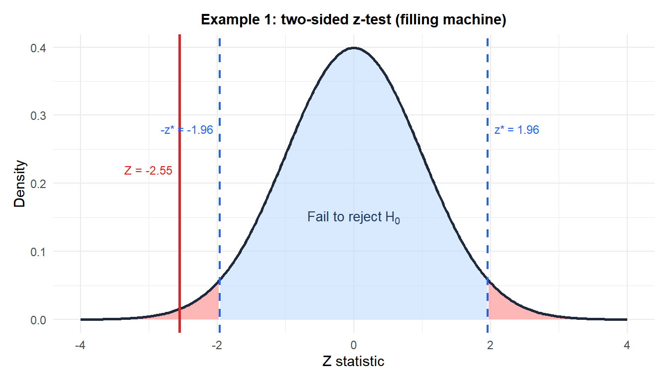
Example 1: quality control (two-sided)
A filling machine is calibrated to dispense \(\mu_0 = 500\) ml per bottle. The machine’s variability is well-established from years of production records: \(\sigma = 4\) ml. A quality engineer samples 36 bottles and finds \(\bar{x} = 498.3\) ml. Has the calibration drifted?
Hypotheses: \(H_0: \mu = 500\) vs \(H_1: \mu \neq 500\).
Test statistic:
\[Z = \frac{498.3 - 500}{4/\sqrt{36}} = \frac{-1.7}{0.667} \approx -2.550\]
p-value (two-sided):
\[p = 2 \times P(Z \leq -2.550) = 2 \times 0.0054 = 0.011\]
Decision: \(p = 0.011 < 0.05\), reject \(H_0\).
The machine’s output has drifted significantly below the target. Recalibration is needed.
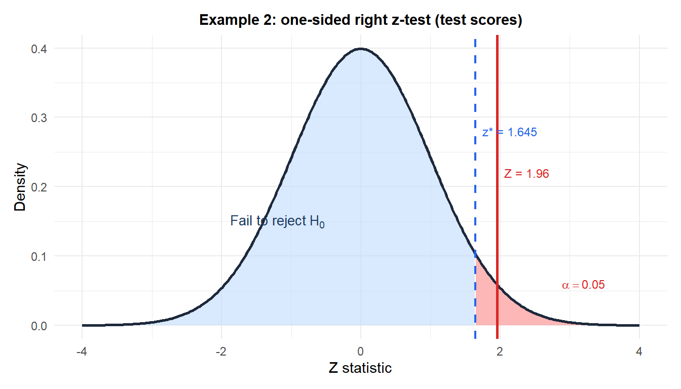
Example 2: standardized test scores (one-sided right)
A national standardized test has a known population standard deviation of \(\sigma = 15\) points (established from millions of past administrations). A school district tests 49 students after implementing a new curriculum and finds \(\bar{x} = 104.2\). Is there evidence that the curriculum improved scores above the national mean of \(\mu_0 = 100\)?
Hypotheses: \(H_0: \mu = 100\) vs \(H_1: \mu > 100\).
Test statistic:
\[Z = \frac{104.2 - 100}{15/\sqrt{49}} = \frac{4.2}{2.143} \approx 1.960\]
p-value (one-sided right):
\[p = P(Z \geq 1.960) = 0.025\]
Decision: \(p = 0.025 < 0.05\), reject \(H_0\).
There is significant evidence at the 5% level that the new curriculum improved scores above the national mean.
Connection with the confidence interval
When \(\sigma\) is known, the \((1-\alpha)\) CI for \(\mu\) uses \(z_{\alpha/2}\) instead of \(t_{\alpha/2,n-1}\):
\[\bar{x} \pm z_{\alpha/2} \cdot \frac{\sigma}{\sqrt{n}}\]
For Example 1: \(498.3 \pm 1.96 \times 4/\sqrt{36} = 498.3 \pm 1.307 = (496.99,\; 499.61)\).
Since \(\mu_0 = 500\) falls outside this interval, the two-sided test rejects \(H_0\) at the 5% level, consistent with \(p = 0.011\).
Running the test in R
Base R does not have a dedicated z.test() function since the \(t\)-test covers all practical cases. For the rare situations where \(\sigma\) is truly known:
# Manual z-test
x_bar <- 498.3
mu0   <- 500
sigma <- 4
n     <- 36

z_stat <- (x_bar - mu0) / (sigma / sqrt(n))
p_two  <- 2 * pnorm(-abs(z_stat))   # two-sided
p_one  <- pnorm(z_stat)              # one-sided left

# The BSDA package provides z.test()
library(BSDA)
z.test(x, mu = 500, sigma.x = 4, alternative = "two.sided")
💡 z-test vs t-test: the practical rule
- \(\sigma\) unknown → always use
t.test(). This is the case in virtually all real applications. - \(\sigma\) known from a very large historical baseline (thousands of observations) → z-test is acceptable.
- Large \(n\) (\(\geq 100\)) and \(\sigma\) unknown → \(t\)-test and z-test give nearly identical results, but \(t\)-test is still correct.
The z-test is mostly useful for teaching the logic of hypothesis testing: it uses the simpler standard normal distribution and avoids the complication of degrees of freedom.

