Welch's t-test
Welch’s t-test compares the means of two independent groups without assuming that their population variances are equal. It is the correct default for two-sample comparisons: it performs almost as well as the pooled t-test when variances are equal, and substantially better when they are not.
Hypotheses
| Test | \(H_0\) | \(H_1\) |
|---|---|---|
| Two-sided | \(\mu_1 = \mu_2\) | \(\mu_1 \neq \mu_2\) |
| One-sided right | \(\mu_1 = \mu_2\) | \(\mu_1 > \mu_2\) |
| One-sided left | \(\mu_1 = \mu_2\) | \(\mu_1 < \mu_2\) |
Test statistic
Given two independent samples with means \(\bar{x}_1\), \(\bar{x}_2\), variances \(S_1^2\), \(S_2^2\), and sizes \(n_1\), \(n_2\):
\[t = \frac{\bar{x}_1 - \bar{x}_2}{\sqrt{\dfrac{S_1^2}{n_1} + \dfrac{S_2^2}{n_2}}}\]
The degrees of freedom are given by the Satterthwaite approximation:
\[df = \frac{\left(\dfrac{S_1^2}{n_1} + \dfrac{S_2^2}{n_2}\right)^2}{\dfrac{(S_1^2/n_1)^2}{n_1-1} + \dfrac{(S_2^2/n_2)^2}{n_2-1}}\]
This is generally not an integer and is rounded down. It is always less than or equal to \(n_1 + n_2 - 2\) (the pooled degrees of freedom), making Welch slightly more conservative when variances are equal.
Welch vs pooled t-test
The pooled t-test assumes \(\sigma_1^2 = \sigma_2^2\) and estimates the common variance as:
\[S_p^2 = \frac{(n_1-1)S_1^2 + (n_2-1)S_2^2}{n_1+n_2-2}\]
giving \(df = n_1+n_2-2\). When variances are truly equal, the pooled test is slightly more powerful. When they differ, the pooled test can be anticonservative: it rejects \(H_0\) more often than it should.
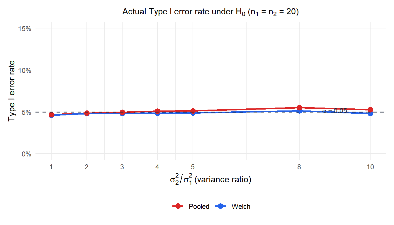
Welch’s test (blue) maintains the nominal 5% Type I error rate regardless of the variance ratio. The pooled test (red) inflates above 5% as soon as the variances differ, reaching over 10% when the variance ratio is 10.
⚠️ Do not use the F-test to decide between Welch and pooled
A common but incorrect workflow: first test \(H_0: \sigma_1^2 = \sigma_2^2\) with the F-test, and if not rejected use the pooled t-test, otherwise use Welch. This is problematic for two reasons:
- The F-test for variances has low power for small samples: it often fails to detect real variance differences, leading you to incorrectly use the pooled test.
- The two-stage procedure distorts the actual significance level of the final t-test.
The correct approach: always use Welch by default. If variances happen to be equal, Welch loses almost no power. If they differ, Welch is correct and pooled is not. This is why t.test() in R uses var.equal = FALSE by default.
Examples
Example 1: delivery times by courier (two-sided)
A logistics manager compares delivery times between two couriers. Courier A (\(n_1 = 30\)): \(\bar{x}_1 = 2.8\) days, \(S_1 = 0.6\) days. Courier B (\(n_2 = 25\)): \(\bar{x}_2 = 3.2\) days, \(S_2 = 1.4\) days.
Test statistic:
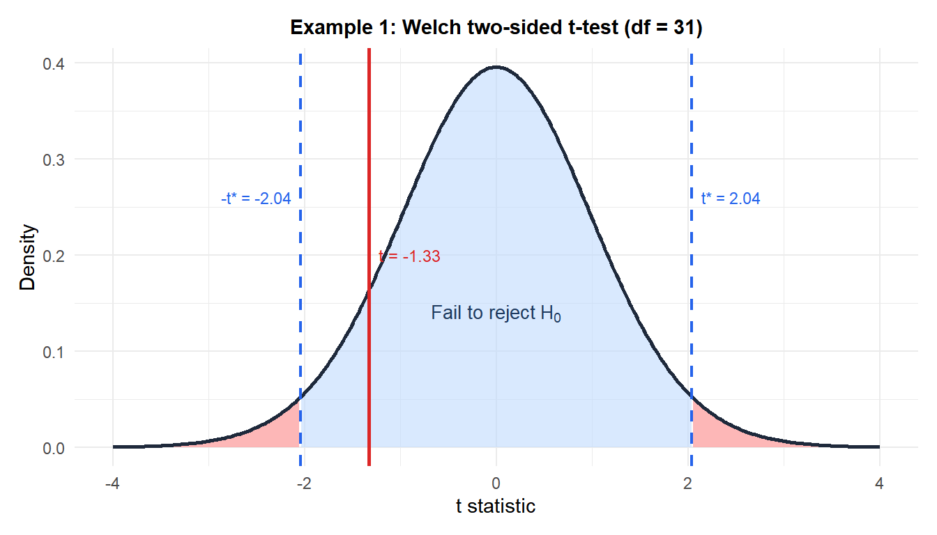
\[t = \frac{2.8 - 3.2}{\sqrt{0.36/30 + 1.96/25}} = \frac{-0.4}{\sqrt{0.012 + 0.0784}} = \frac{-0.4}{\sqrt{0.0904}} = \frac{-0.4}{0.3007} \approx -1.330\]
Satterthwaite df:
\[df = \frac{(0.012 + 0.0784)^2}{(0.012)^2/29 + (0.0784)^2/24} = \frac{0.008156}{0.00000497 + 0.000256} \approx 31.1 \to 31\]
p-value (two-sided): \(p = 2 \times P(T_{31} \leq -1.330) \approx 0.193\).
Decision: \(p = 0.193 > 0.05\), fail to reject \(H_0\). No significant difference in mean delivery time between the two couriers.
Example 2: drug vs placebo (one-sided right)
A clinical trial measures blood pressure reduction (mmHg). Treatment (\(n_1 = 40\)): \(\bar{x}_1 = 14.2\), \(S_1 = 5.8\). Placebo (\(n_2 = 38\)): \(\bar{x}_2 = 10.9\), \(S_2 = 3.1\).
Test statistic:
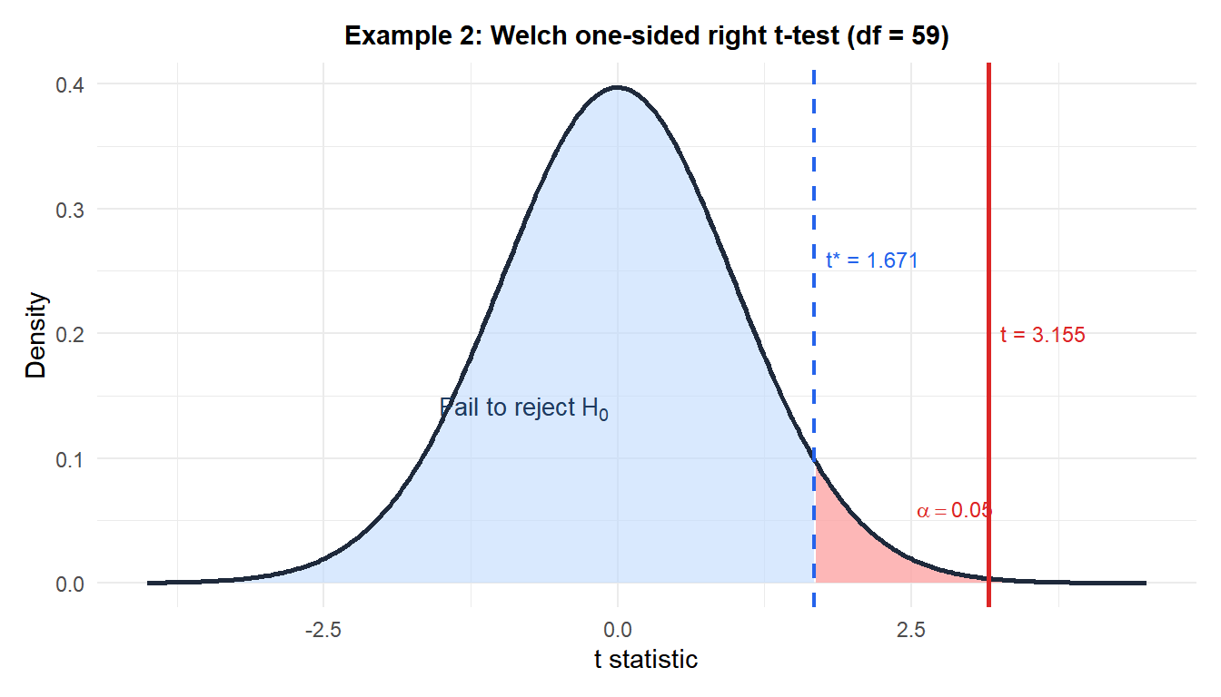
\[t = \frac{14.2 - 10.9}{\sqrt{33.64/40 + 9.61/38}} = \frac{3.3}{\sqrt{0.841 + 0.253}} = \frac{3.3}{\sqrt{1.094}} = \frac{3.3}{1.046} \approx 3.155\]
Satterthwaite df \(\approx 59\) (computed by software).
p-value (one-sided right): \(p = P(T_{59} \geq 3.155) \approx 0.001\).
Decision: \(p = 0.001 < 0.05\), reject \(H_0\). The drug produces significantly greater blood pressure reduction than placebo.
Running the test in R
Welch’s t-test is the default in R:
# Welch t-test (default, var.equal = FALSE)
t.test(x1, x2, alternative = "two.sided")
t.test(x1, x2, alternative = "greater")

# Pooled t-test (requires equal variance assumption)
t.test(x1, x2, var.equal = TRUE)

# Formula interface for data frames
t.test(value ~ group, data = df, alternative = "two.sided")
The output includes the t statistic, Satterthwaite df, p-value, and a 95% CI for \(\mu_1 - \mu_2\).
💡 Reporting the result
Always report the mean difference and its confidence interval alongside the test result. For Example 2: “The treatment reduced blood pressure by 3.3 mmHg more than placebo (95% CI: 1.2 to 5.4 mmHg; Welch’s \(t_{59} = 3.155\), \(p = 0.001\)).” This gives both the statistical significance and the practical magnitude of the effect.

