Steps for a Hypothesis Test

The steps of hypothesis testing are the same across all tests: state the hypotheses, set \(\alpha\), choose the test, compute the statistic and p-value, decide, and interpret. What changes between tests is the formula for the statistic and the reference distribution. This post works through three complete examples to show how to apply the steps in practice.

The six steps

Every hypothesis test follows the same structure:

1. State \(H_0\) and \(H_1\): define what you are testing and the direction of the alternative.

2. Set \(\alpha\): choose the significance level before seeing the data. Common choices: 0.05 and 0.01.

3. Choose the test and compute the statistic: select the appropriate test for your data type and sample size, then compute the test statistic from the sample.

4. Compute the p-value: the probability of observing a statistic at least as extreme as the one computed, assuming \(H_0\) is true.

5. Decide: if \(p \leq \alpha\), reject \(H_0\). If \(p > \alpha\), fail to reject \(H_0\).

6. Interpret in context: translate the statistical decision into a practical conclusion.

The rest of this post applies these steps to three real examples.

Example 1: one-sample t-test

A logistics company claims their average delivery time is 48 hours. A customer rights organization samples 25 deliveries and finds \(\bar{x} = 51.3\) hours and \(S = 8.4\) hours.

Step 1: hypotheses

\[H_0: \mu = 48 \quad \text{vs} \quad H_1: \mu > 48 \quad \text{(one-sided, right)}\]

The organization suspects deliveries take longer than claimed, so the alternative is one-sided to the right.

Step 2: significance level

\[\alpha = 0.05\]

Step 3: test statistic

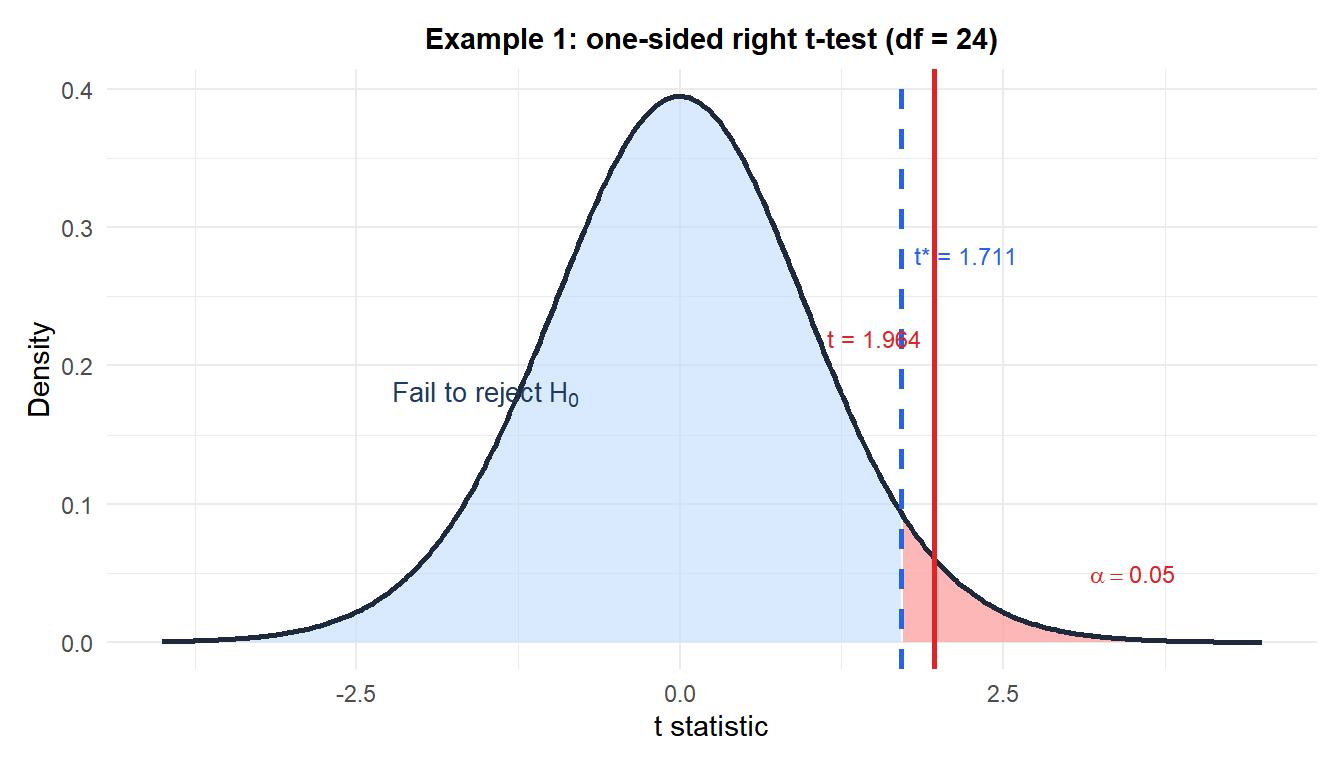
Population \(\sigma\) is unknown and \(n = 25\): use a one-sample \(t\)-test.

\[t = \frac{\bar{x} - \mu_0}{S/\sqrt{n}} = \frac{51.3 - 48}{8.4/\sqrt{25}} = \frac{3.3}{1.68} \approx 1.964\]

Step 4: p-value

With \(df = 24\) and a one-sided right test:

\[p = P(T_{24} > 1.964) \approx 0.031\]

Steps 5 and 6: decision and interpretation

Since \(p = 0.031 < 0.05\), reject \(H_0\).

There is significant evidence at the 5% level that the true average delivery time exceeds 48 hours. The company’s claim appears to be understated by the data.

Example 2: one-sample proportion test

An e-commerce platform claims their checkout process has a cart abandonment rate of 70%. An analyst samples 200 sessions and observes 152 abandonments (76%).

Step 1: hypotheses

\[H_0: p = 0.70 \quad \text{vs} \quad H_1: p \neq 0.70 \quad \text{(two-sided)}\]

Step 2: significance level

\[\alpha = 0.05\]

Step 3: test statistic

Check: \(np_0 = 200 \times 0.70 = 140 \geq 10\) and \(n(1-p_0) = 60 \geq 10\). Use the z-test for proportions.

\[z = \frac{\hat{p} - p_0}{\sqrt{p_0(1-p_0)/n}} = \frac{0.76 - 0.70}{\sqrt{0.70 \times 0.30/200}} = \frac{0.06}{0.0324} \approx 1.852\]

Step 4: p-value

Two-sided: \(p = 2 \times P(Z > 1.852) = 2 \times 0.032 = 0.064\).

Steps 5 and 6: decision and interpretation

Since \(p = 0.064 > 0.05\), fail to reject \(H_0\).

The observed abandonment rate of 76% is not significantly different from the claimed 70% at the 5% level. The data are compatible with the platform’s claim, though the result is borderline (\(p = 0.064\)). A larger sample would give a more definitive answer.

What changes with α = 0.10?

If the analyst had set \(\alpha = 0.10\) instead of \(\alpha = 0.05\), the critical value would be \(z_{0.05} = 1.645\). Since \(z = 1.852 > 1.645\), \(H_0\) would be rejected at the 10% level.

This illustrates why \(\alpha\) must be chosen before seeing the data. Adjusting \(\alpha\) after computing the p-value to achieve a desired conclusion is p-hacking.

Example 3: two-sample t-test

A clinical trial compares blood pressure reduction (mmHg) between two treatments. Treatment A (\(n_1 = 30\)): \(\bar{x}_1 = 12.4\), \(S_1 = 4.2\). Treatment B (\(n_2 = 28\)): \(\bar{x}_2 = 10.1\), \(S_2 = 5.1\).

Step 1: hypotheses

\[H_0: \mu_1 - \mu_2 = 0 \quad \text{vs} \quad H_1: \mu_1 - \mu_2 \neq 0 \quad \text{(two-sided)}\]

Step 2: significance level

\[\alpha = 0.05\]

Step 3: test statistic (Welch)

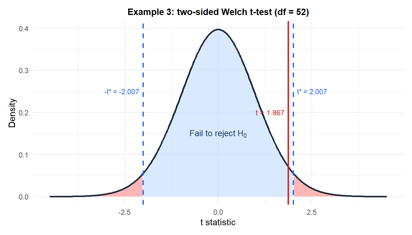
Variances differ (\(S_1 \neq S_2\)), so use Welch’s \(t\)-test.

\[\text{SE} = \sqrt{\frac{4.2^2}{30} + \frac{5.1^2}{28}} = \sqrt{0.588 + 0.929} = \sqrt{1.517} \approx 1.232\]

\[t = \frac{12.4 - 10.1}{1.232} \approx 1.867\]

Satterthwaite degrees of freedom: \(df \approx 52\).

Step 4: p-value

\[p = 2 \times P(T_{52} > 1.867) \approx 2 \times 0.034 = 0.068\]

Steps 5 and 6: decision and interpretation

Since \(p = 0.068 > 0.05\), fail to reject \(H_0\).

The data do not provide significant evidence at the 5% level that the two treatments differ. However, \(p = 0.068\) is close to the threshold: the study may be underpowered. With larger samples, the observed difference of 2.3 mmHg might reach significance.