The P-Value
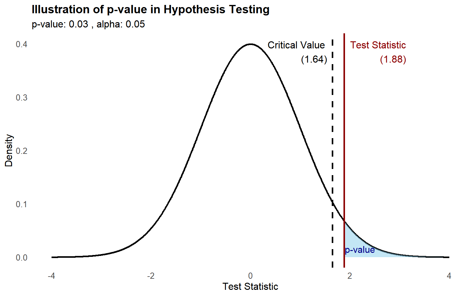
The p-value is the probability of observing data at least as extreme as what was obtained, assuming the null hypothesis is true. It is the most widely reported quantity in statistics and the most widely misinterpreted.
Definition
Given a test statistic computed from the data, the p-value is:
\[p = P(\text{test statistic as extreme or more extreme than observed} \mid H_0 \text{ true})\]
“More extreme” means further from what \(H_0\) predicts:
- One-sided right (\(H_1: \theta > \theta_0\)): more extreme = larger values. \(p = P(T \geq t_\text{obs})\).
- One-sided left (\(H_1: \theta < \theta_0\)): more extreme = smaller values. \(p = P(T \leq t_\text{obs})\).
- Two-sided (\(H_1: \theta \neq \theta_0\)): more extreme in either direction. \(p = 2 \times P(T \geq |t_\text{obs}|)\).
P-value in one-sided vs two-sided tests
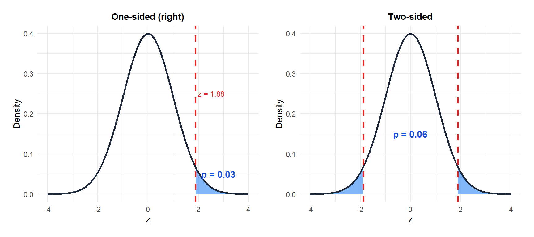
The same test statistic produces different p-values depending on the direction of \(H_1\). For a standard normal with \(z_\text{obs} = 1.88\):
- One-sided right: \(p = P(Z \geq 1.88) \approx 0.030\).
- Two-sided: \(p = 2 \times P(Z \geq 1.88) \approx 0.060\).
The two-sided p-value is exactly double the one-sided. This is why a result significant at 5% one-sided may not be significant at 5% two-sided.
How to interpret the p-value
The decision rule is simple: if \(p \leq \alpha\), reject \(H_0\). If \(p > \alpha\), fail to reject \(H_0\).
But interpreting what the p-value means requires more care:
- Small p-value: the observed data would be unlikely if \(H_0\) were true. This is evidence against \(H_0\).
- Large p-value: the observed data are compatible with \(H_0\). This is not evidence in favor of \(H_0\).
A useful mental model: the p-value is a surprise index. A very small p-value means “this result would be very surprising if \(H_0\) were true.” It does not measure how surprising it is given any alternative.
Common misconceptions
- “The p-value is the probability that \(H_0\) is true”
This is the most dangerous misconception. The p-value is computed under the assumption that \(H_0\) is true. It cannot say anything about the probability of \(H_0\) being true, because that would require a prior probability for \(H_0\) (which is a Bayesian concept, not a frequentist one).
A test gives \(p = 0.03\). This does not mean there is a 3% chance \(H_0\) is true. It means: if \(H_0\) were true, there would be a 3% chance of seeing data this extreme. These two statements are completely different.
To calculate the probability that \(H_0\) is true given the data, you need Bayes’ theorem and a prior for \(H_0\), which frequentist hypothesis testing deliberately avoids.
- “\(p < 0.05\) proves \(H_1\) is true”
A low p-value means the data are inconsistent with \(H_0\), not that \(H_1\) is proven. Multiple different alternative hypotheses could be consistent with the same data. Statistical significance is not the same as proof.
- “\(p > 0.05\) means \(H_0\) is true”
Failing to reject \(H_0\) means the data are compatible with \(H_0\), not that \(H_0\) is confirmed. The data may simply be insufficient to detect a real effect. Absence of evidence is not evidence of absence.
- “Statistical significance means practical importance”
With large enough samples, even trivially small effects produce tiny p-values. A drug that reduces blood pressure by 0.1 mmHg can be highly statistically significant in a trial with 100,000 patients but completely irrelevant clinically. Always pair p-values with effect sizes and confidence intervals.
⚠️ The p-value threshold of 0.05 is arbitrary
The 0.05 threshold was proposed by R.A. Fisher in 1925 as a convenient rule of thumb, not a fundamental law. It has no special scientific meaning. A result with \(p = 0.049\) is not meaningfully different from one with \(p = 0.051\): both provide similar evidence against \(H_0\).
Many scientific journals and the American Statistical Association now recommend reporting the exact p-value and the effect size rather than making binary significant/not-significant decisions. Treat the p-value as a continuous measure of evidence, not a bright line.
Worked example
An online retailer runs an A/B test on two button colors. Version A (blue): 1,240 clicks out of 8,000 impressions. Version B (green): 1,380 clicks out of 8,000 impressions.
\[\hat{p}_A = 0.155, \quad \hat{p}_B = 0.1725, \quad \hat{p}_A - \hat{p}_B = -0.0175\]
\[\text{SE} = \sqrt{\frac{0.155 \times 0.845}{8000} + \frac{0.1725 \times 0.8275}{8000}} \approx 0.00573\]
\[z = \frac{-0.0175}{0.00573} \approx -3.05\]
\[p = 2 \times P(Z \leq -3.05) \approx 2 \times 0.00114 = 0.0023\]
The p-value is 0.0023, far below \(\alpha = 0.05\). This is strong evidence that the two conversion rates differ. Version B converts at a meaningfully higher rate.
The effect size: Version B converts 1.75 percentage points more than Version A, a relative improvement of about 11%. Both the p-value (significant) and the effect size (meaningful for the business) support switching to Version B.
💡 Reporting p-values correctly
- Report the exact p-value, not just “\(p < 0.05\)”: write “\(p = 0.023\)”, not “\(p < 0.05\)”.
- Always report the effect size alongside the p-value.
- If the p-value is very small, write “\(p < 0.001\)” rather than “\(p = 0.0000023\)”.
- Never adjust \(\alpha\) after computing the p-value to achieve significance.
- For borderline results (\(p\) near \(\alpha\)), state that the evidence is not conclusive and suggest larger samples.

