Jarque-Bera test
The Jarque-Bera test evaluates normality by checking two specific properties: skewness (symmetry) and excess kurtosis (tail weight). A normal distribution has skewness 0 and excess kurtosis 0. The test quantifies how far the sample departs from both, and combines them into a single chi-squared statistic.
Test statistic
\[JB = \frac{n}{6}\left(S^2 + \frac{(K-3)^2}{4}\right)\]
where \(n\) is the sample size, \(S\) is the sample skewness, and \(K\) is the sample excess kurtosis (so a normal distribution gives \(K-3 = 0\)). Under \(H_0\) (normality), \(JB\) follows a \(\chi^2\) distribution with 2 degrees of freedom for large \(n\).
The two terms are the two components of the test:
- \(S^2\): contribution from skewness. A skewed distribution increases this term.
- \((K-3)^2/4\): contribution from excess kurtosis. Heavy or light tails increase this term.
Hypotheses: \(H_0\): the data are normally distributed (\(S = 0\) and \(K = 3\)). \(H_1\): skewness and/or kurtosis deviate from normal values.
Decomposing non-normality
The JB test is unique among normality tests in that it tells you not just whether the data are non-normal, but in which way: via skewness, kurtosis, or both.
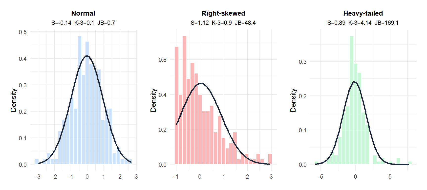
The normal data has \(S \approx 0\) and \(K-3 \approx 0\), giving a small JB. The skewed data has high \(|S|\), driven by asymmetry. The heavy-tailed data has high \(|K-3|\), driven by excess kurtosis, even if roughly symmetric.
Step-by-step example
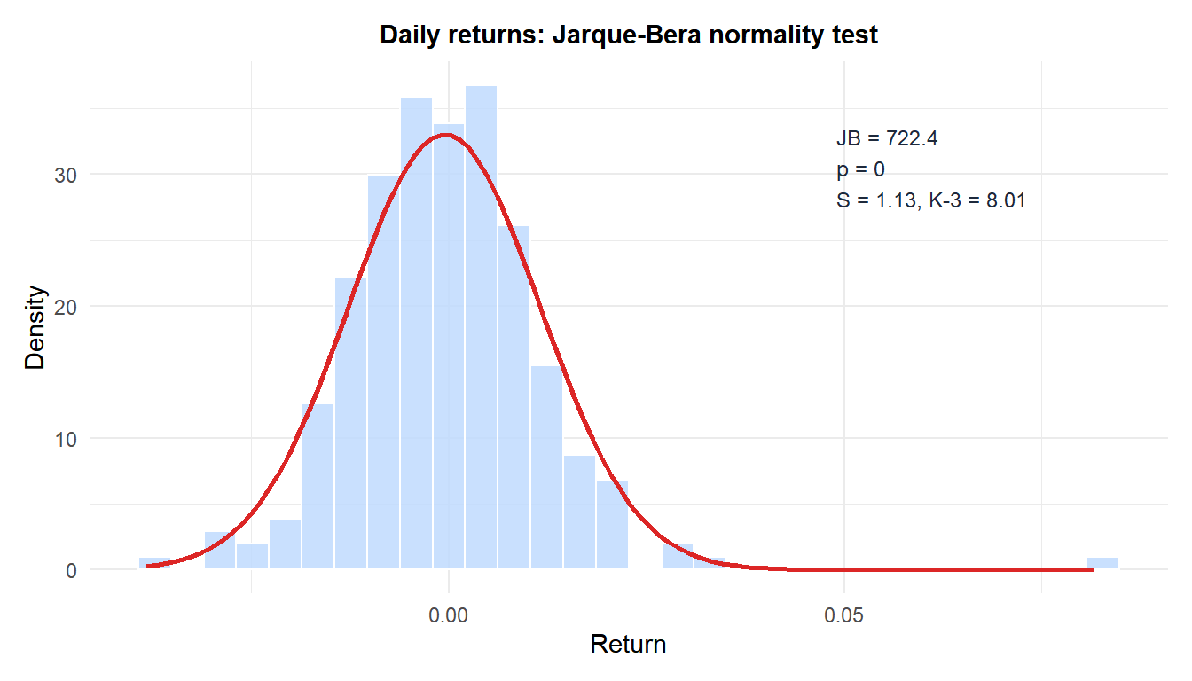
A financial analyst tests whether daily stock returns (\(n = 250\)) follow a normal distribution. The sample gives \(S = 0.61\) (mild right skew) and \(K = 4.82\) (slightly heavy tails, so \(K - 3 = 1.82\)).
Test statistic:
\[JB = \frac{250}{6}\left(0.61^2 + \frac{1.82^2}{4}\right) = 41.67 \times \left(0.372 + 0.828\right) = 41.67 \times 1.200 = 50.0\]
Critical value (\(\chi^2_{0.05, 2} = 5.991\)) and p-value (\(p \approx 0.000\)).
Decision: reject \(H_0\). The returns are significantly non-normal, with contributions from both skewness and excess kurtosis. This is typical of financial returns, which tend to be leptokurtic (fat tails) and slightly skewed.
Assumptions and limitations
⚠️ The chi-squared approximation is unreliable for small samples
The \(\chi^2(2)\) p-value is only accurate for large samples. For \(n < 30\), the actual distribution of \(JB\) under \(H_0\) differs substantially from \(\chi^2(2)\), making p-values unreliable. For \(n < 100\), the approximation is still imperfect.
For small samples, use Shapiro-Wilk instead. The JB test is best suited for \(n \geq 100\), where it provides good power against both skewness and kurtosis departures.
⚠️ The test only captures skewness and kurtosis departures
The JB test is blind to departures from normality that do not manifest as changes in skewness or kurtosis. For example, a bimodal distribution with equal-sized symmetric modes can have \(S = 0\) and \(K \approx 3\), passing the JB test despite being clearly non-normal. Use a Q-Q plot alongside the formal test.
When to use JB vs Shapiro-Wilk
| Criterion | Jarque-Bera | Shapiro-Wilk |
|---|---|---|
| Best sample size | \(n \geq 100\) | \(3 \leq n \leq 5000\) |
| Power for small \(n\) | Low | High |
| Identifies departure type | Yes (skewness vs kurtosis) | No |
| Used in econometrics | Very common | Less common |
| R function | tseries::jarque.bera.test() |
shapiro.test() |
The JB test is standard in econometrics and finance, where large samples are common and interest in fat tails is high. For general statistics, Shapiro-Wilk is usually preferred.
Running the test in R
The JB test is available in the tseries and moments packages. Both give the same result:
library(tseries)
jarque.bera.test(x)

# Or manually:
library(moments)
n <- length(x)
S <- skewness(x)
K <- kurtosis(x)   # moments uses excess kurtosis by default
JB <- n/6 * (S^2 + (K - 3)^2 / 4)
p_val <- pchisq(JB, df = 2, lower.tail = FALSE)
💡 Practical workflow for normality in large samples
For \(n \geq 100\) where Shapiro-Wilk may be overpowered:
- Plot a histogram and Q-Q plot to visually assess the departure.
- Run the JB test to get a formal p-value.
- If rejected, check which component (\(S\) or \(K-3\)) drives the result: this guides the choice of remedy (transformation for skewness, robust methods or heavy-tailed distributions for kurtosis).
- Consider whether the downstream test is robust to the specific type of non-normality detected.

