What is a hypothesis test?
A hypothesis test uses sample data to evaluate a claim about a population parameter. It does not prove or disprove anything with certainty: it quantifies how compatible the data are with the null hypothesis, and provides a structured framework for making decisions under uncertainty.
The two hypotheses
Every hypothesis test starts with two competing statements about a population parameter:
- The null hypothesis \(H_0\): the default position, usually “no effect”, “no difference”, or a specific value. It is assumed true until the data provide sufficient evidence against it.
- The alternative hypothesis \(H_1\) (or \(H_a\)): the claim we want to assess. It is accepted only when the data are inconsistent with \(H_0\).
A manufacturer claims their batteries last 20 hours on average. A consumer group suspects the true average is lower.
- \(H_0\): \(\mu = 20\) hours (the claim is correct).
- \(H_1\): \(\mu < 20\) hours (the batteries last less than claimed).
A pharmaceutical company tests a new drug against placebo.
- \(H_0\): \(\mu_{\text{drug}} - \mu_{\text{placebo}} = 0\) (no effect).
- \(H_1\): \(\mu_{\text{drug}} - \mu_{\text{placebo}} \neq 0\) (some effect, either direction).
One-sided vs two-sided tests
The choice of \(H_1\) determines the test direction:
- Two-sided (\(H_1: \theta \neq \theta_0\)): reject \(H_0\) if the statistic is extreme in either direction. Use when you have no prior reason to expect a specific direction.
- One-sided (\(H_1: \theta > \theta_0\) or \(H_1: \theta < \theta_0\)): reject only in one tail. Use when only one direction is scientifically or practically meaningful.
⚠️ Choose the test direction before seeing the data
The direction of \(H_1\) must be specified based on the research question, not based on what the data show. Switching from a two-sided to a one-sided test after seeing that the result is in the “right” direction halves the p-value but is not valid: it is a form of p-hacking. Pre-register your hypotheses or use two-sided tests by default when in doubt.
Steps in hypothesis testing
Step 1: state the hypotheses \(H_0\) and \(H_1\).
Step 2: choose \(\alpha\), the significance level. Common choices are 0.05 and 0.01. This is the maximum acceptable probability of a Type I error (rejecting \(H_0\) when it is true).
Step 3: compute the test statistic, a function of the sample data that measures how far the observed data are from what \(H_0\) predicts. For a one-sample \(t\)-test:
\[t = \frac{\bar{X} - \mu_0}{S/\sqrt{n}}\]
Step 4: compute the p-value (or compare to a critical value). The p-value is the probability of observing a test statistic at least as extreme as the one computed, assuming \(H_0\) is true.
Step 5: make a decision. If \(p \leq \alpha\), reject \(H_0\). If \(p > \alpha\), fail to reject \(H_0\).
Step 6: interpret in context. A statistical decision is not the end: translate it into a practical conclusion.
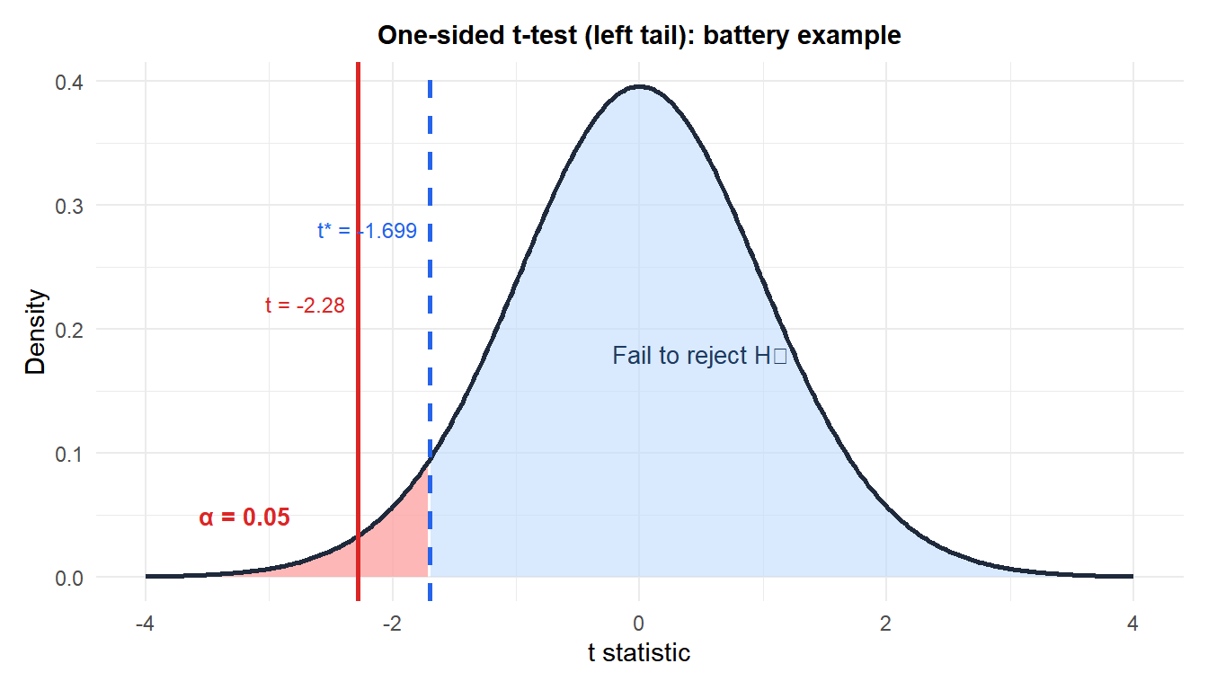
The red line is the observed \(t = -2.28\), which falls in the rejection region (red area). Since \(t < t^* = -1.699\), we reject \(H_0\).
The p-value
The p-value is the probability, computed under \(H_0\), of observing a test statistic at least as extreme as the one obtained.
⚠️ The p-value is not the probability that H0 is true
The most common misinterpretation: “the p-value is the probability that the null hypothesis is true.” This is wrong.
- Correct: the p-value is \(P(\text{data this extreme or more} \mid H_0 \text{ is true})\).
- Wrong: the p-value is \(P(H_0 \text{ is true} \mid \text{data})\).
These are completely different quantities. The p-value is a frequentist concept: it says nothing about the probability of any hypothesis. A small p-value means the data are unlikely under \(H_0\), not that \(H_0\) is unlikely.
A second common error: “a p-value of 0.03 means there is a 3% chance we are wrong.” Also incorrect. The p-value is computed assuming \(H_0\) is true; it cannot be interpreted as an error probability for any specific conclusion.
⚠️ Statistical significance is not practical significance
A result can be statistically significant (\(p < 0.05\)) but practically irrelevant, especially with large samples. With \(n = 10{,}000\), a difference of 0.001 units might be highly significant but completely unimportant in practice.
Always report effect sizes alongside p-values: Cohen’s \(d\), relative risk, or the confidence interval for the parameter. The CI tells you both whether the effect is significant and how large it is.
Type I and Type II errors
Two types of error are possible in any hypothesis test:
| \(H_0\) true | \(H_0\) false | |
|---|---|---|
| Reject \(H_0\) | Type I error (\(\alpha\)) | Correct (power \(= 1-\beta\)) |
| Fail to reject \(H_0\) | Correct | Type II error (\(\beta\)) |
- Type I error (false positive): reject \(H_0\) when it is true. Probability \(= \alpha\), controlled by the significance level.
- Type II error (false negative): fail to reject \(H_0\) when it is false. Probability \(= \beta\).
- Power \(= 1 - \beta\): probability of correctly rejecting a false \(H_0\).
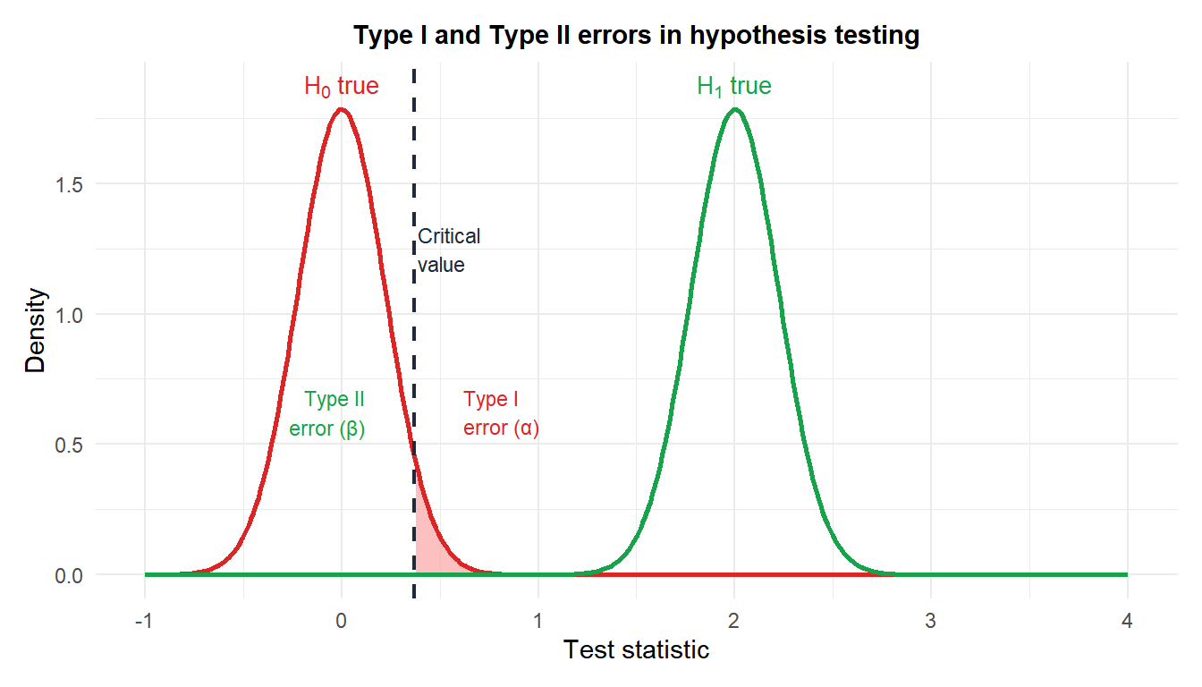
The tradeoff: decreasing \(\alpha\) (moving the critical value right) reduces Type I errors but increases Type II errors (\(\beta\)). For fixed \(\alpha\), increasing \(n\) reduces both errors simultaneously.
Complete example: battery lifetime
A manufacturer claims their batteries last \(\mu_0 = 20\) hours. A researcher samples 30 batteries and finds \(\bar{x} = 19.5\) hours, \(S = 1.2\) hours. Test at \(\alpha = 0.05\).
Hypotheses: \(H_0: \mu = 20\) vs \(H_1: \mu < 20\) (one-sided, left).
Test statistic:
\[t = \frac{19.5 - 20}{1.2/\sqrt{30}} = \frac{-0.5}{0.219} \approx -2.28\]
Critical value: \(t_{0.05,\; 29} = -1.699\).
p-value: \(P(T_{29} < -2.28) \approx 0.015\).
Decision: since \(t = -2.28 < -1.699\) and \(p = 0.015 < 0.05\), reject \(H_0\).
Conclusion: there is significant evidence at the 5% level that the average battery life is less than 20 hours. The manufacturer’s claim appears to be overstated.
Sample size and power
Power is the probability of rejecting \(H_0\) when \(H_1\) is true. For a one-sample \(t\)-test detecting a difference \(\delta = \mu_1 - \mu_0\) with known \(\sigma\):
\[n \geq \frac{(z_{\alpha} + z_{\beta})^2 \sigma^2}{\delta^2}\]
For the battery example: suppose the true mean is \(\mu_1 = 19.5\) hours (\(\delta = 0.5\)), \(\sigma = 1.2\), \(\alpha = 0.05\), desired power \(= 0.80\) (\(z_\beta = 0.842\)):
\[n \geq \frac{(1.645 + 0.842)^2 \times 1.44}{0.25} = \frac{6.185 \times 1.44}{0.25} = \frac{8.91}{0.25} \approx 36\]
With \(n = 30\) (the actual sample), power is slightly below 80%, which explains why the test barely rejected \(H_0\).
💡 Practical guidelines
- Always specify \(H_0\), \(H_1\), \(\alpha\), and the test before collecting data.
- Report the p-value and the effect size, not just “significant” or “not significant”.
- A two-sided test is the safe default unless there is a clear directional hypothesis stated in advance.
- For a new study, calculate the required \(n\) to achieve at least 80% power before collecting data.
- \(p > 0.05\) does not mean \(H_0\) is true: it means the data do not provide enough evidence to reject it. The absence of evidence is not evidence of absence.

