Hypothesis testing for a mean
The one-sample test for a mean evaluates whether a population mean equals a specific hypothesized value. The \(t\)-test is the standard tool whenever \(\sigma\) is unknown, which is almost always the case in practice.
Hypotheses
The null hypothesis specifies a value \(\mu_0\) for the population mean. The alternative depends on the research question:
| Test | \(H_0\) | \(H_1\) |
|---|---|---|
| Two-sided | \(\mu = \mu_0\) | \(\mu \neq \mu_0\) |
| One-sided right | \(\mu = \mu_0\) | \(\mu > \mu_0\) |
| One-sided left | \(\mu = \mu_0\) | \(\mu < \mu_0\) |
Use a two-sided test by default. Use one-sided only when the research question is directional and that direction was specified before seeing the data.
Test statistic
Given a sample of size \(n\) with mean \(\bar{x}\) and standard deviation \(S\):
\[t = \frac{\bar{x} - \mu_0}{S / \sqrt{n}}\]
Under \(H_0\), this statistic follows a \(t\) distribution with \(n - 1\) degrees of freedom. The p-value is computed from this distribution.
When \(\sigma\) is known (rare in practice), replace \(S\) with \(\sigma\) and use the standard normal \(Z\) instead of \(t\).
⚠️ Always use t when σ is unknown, regardless of sample size
A common but incorrect rule states: “use \(z\) for large samples (\(n > 30\)), use \(t\) for small samples.” This is wrong. The correct rule: use \(t\) whenever \(\sigma\) is estimated from the data, regardless of \(n\).
For large \(n\), \(t\) and \(z\) give virtually identical results, so there is no cost to always using \(t\). For small \(n\), using \(z\) underestimates the uncertainty and produces anticonservative tests.
Assumptions
The one-sample \(t\)-test requires:
- The observations are independent.
- The population is normal, or \(n\) is large enough for the CLT to apply (typically \(n \geq 30\) as a rule of thumb).
For small samples from clearly non-normal populations, consider the Wilcoxon signed-rank test as a non-parametric alternative.
Examples
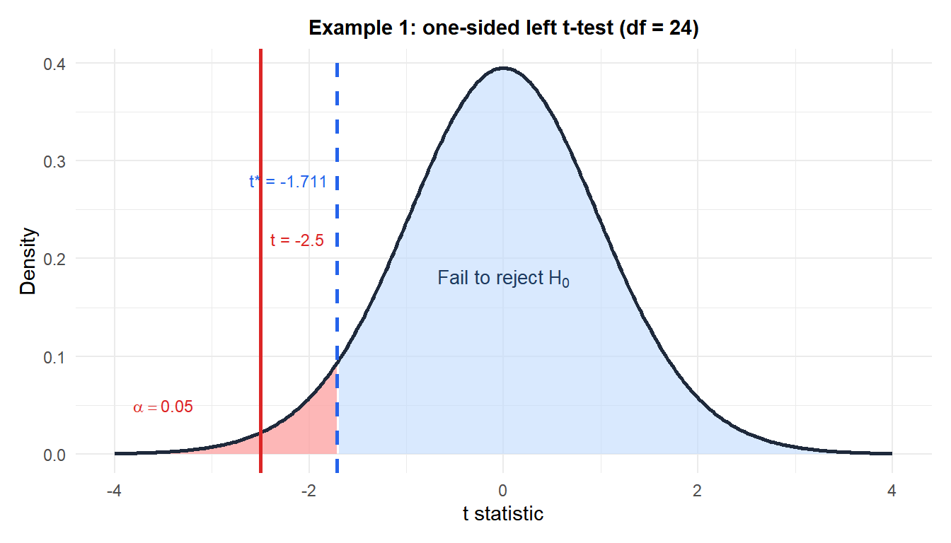
Example 1: product lifetime (one-sided left)
A manufacturer claims their component lasts \(\mu_0 = 10\) years on average. A quality team samples 25 units and finds \(\bar{x} = 9.5\) years, \(S = 1.0\) year. Is there evidence the true mean is less than 10 years?
Hypotheses: \(H_0: \mu = 10\) vs \(H_1: \mu < 10\).
Test statistic:
\[t = \frac{9.5 - 10}{1.0/\sqrt{25}} = \frac{-0.5}{0.2} = -2.500\]
p-value (one-sided left, \(df = 24\)):
\[p = P(T_{24} \leq -2.500) \approx 0.010\]
Decision: \(p = 0.010 < 0.05\), reject \(H_0\).
Conclusion: there is significant evidence at the 5% level that the true average lifetime is less than 10 years. The manufacturer’s claim appears to be overstated.
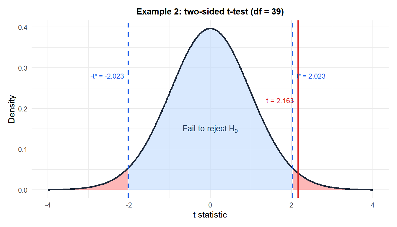
Example 2: server response time (two-sided)
A DevOps team monitors API response time. The SLA requires \(\mu_0 = 200\) ms. After a deployment, they sample 40 requests: \(\bar{x} = 213\) ms, \(S = 38\) ms. Has the mean response time changed?
Hypotheses: \(H_0: \mu = 200\) vs \(H_1: \mu \neq 200\).
Test statistic:
\[t = \frac{213 - 200}{38/\sqrt{40}} = \frac{13}{6.011} \approx 2.163\]
p-value (two-sided, \(df = 39\)):
\[p = 2 \times P(T_{39} \geq 2.163) \approx 2 \times 0.018 = 0.036\]
Decision: \(p = 0.036 < 0.05\), reject \(H_0\).
Conclusion: there is significant evidence that the deployment changed the average response time. The observed increase of 13 ms is statistically significant. The team should investigate whether this degradation is acceptable in practice.
Running the test in R
Both examples can be reproduced with t.test():
# Example 1: one-sided left
t.test(x, mu = 10, alternative = "less")

# Example 2: two-sided
t.test(x, mu = 200, alternative = "two.sided")
The output includes the test statistic, degrees of freedom, p-value, and a 95% confidence interval for \(\mu\).
💡 Interpreting the result
A significant result (\(p \leq \alpha\)) means the data are inconsistent with \(H_0: \mu = \mu_0\). It does not tell you by how much \(\mu\) differs from \(\mu_0\). Always report the confidence interval alongside the test result: the CI shows both the direction and the magnitude of the departure from \(\mu_0\), which is what matters for practical decisions.

