Sample size calculation
Sample size calculation is the step that determines how many observations you need to estimate a parameter with a desired level of precision and confidence. Too small a sample gives an interval too wide to be useful; too large wastes resources. The goal is to find the minimum \(n\) that meets your requirements.
General principle
A confidence interval has the form:
\[\text{estimate} \pm \underbrace{z_{\alpha/2} \cdot \text{SE}}_{\text{margin of error } d}\]
The margin of error \(d\) shrinks as \(n\) grows (since \(\text{SE} \propto 1/\sqrt{n}\)). To achieve a target margin of error \(d\), solve for \(n\). The required sample size always depends on three things:
- The confidence level \((1-\alpha)\): higher confidence requires larger \(n\).
- The margin of error \(d\): smaller \(d\) requires larger \(n\).
- The population variability (\(\sigma\) or \(p\)): more variable populations require larger \(n\).
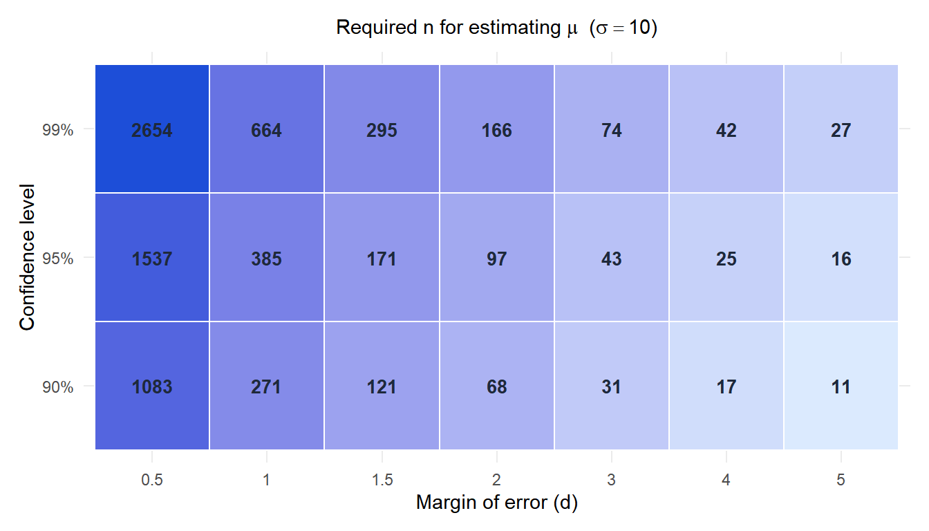
The heatmap shows that small margins of error at high confidence levels demand very large samples. Halving the margin of error quadruples the required \(n\).
Sample size for estimating a mean
To estimate \(\mu\) with margin of error \(d\) at confidence level \(1-\alpha\), when \(\sigma\) is known:
\[n \geq \left(\frac{z_{\alpha/2} \cdot \sigma}{d}\right)^2\]
When \(\sigma\) is unknown, replace it with a pilot estimate \(S\) and use \(t_{\alpha/2, n-1}\) instead of \(z_{\alpha/2}\). Since \(t\) depends on \(n\), iterate: start with \(z\), compute \(n\), then check with \(t_{n-1}\) and adjust if needed.
Common \(z_{\alpha/2}\) values:
| Confidence level | \(z_{\alpha/2}\) |
|---|---|
| 90% | 1.645 |
| 95% | 1.960 |
| 99% | 2.576 |
A hospital wants to estimate the average length of stay for a diagnosis group to within \(\pm 0.5\) days at 95% confidence. From a pilot study, \(S \approx 3.1\) days.
\[n \geq \left(\frac{1.960 \times 3.1}{0.5}\right)^2 = \left(\frac{6.076}{0.5}\right)^2 = 12.152^2 \approx 147.7 \to 148\]
At least 148 patients are needed. If the budget only allows 50 patients, the achievable margin of error would be:
\[d = 1.960 \times \frac{3.1}{\sqrt{50}} \approx 0.86 \text{ days}\]
The hospital must decide whether a margin of \(\pm 0.86\) days is acceptable.
Sample size for estimating a proportion
To estimate \(p\) with margin of error \(d\):
\[n \geq \frac{z_{\alpha/2}^2 \cdot p(1-p)}{d^2}\]
Since \(p\) is unknown, use a prior estimate if available. If not, use \(p = 0.5\), which maximizes \(p(1-p) = 0.25\) and gives the most conservative (largest) sample size.
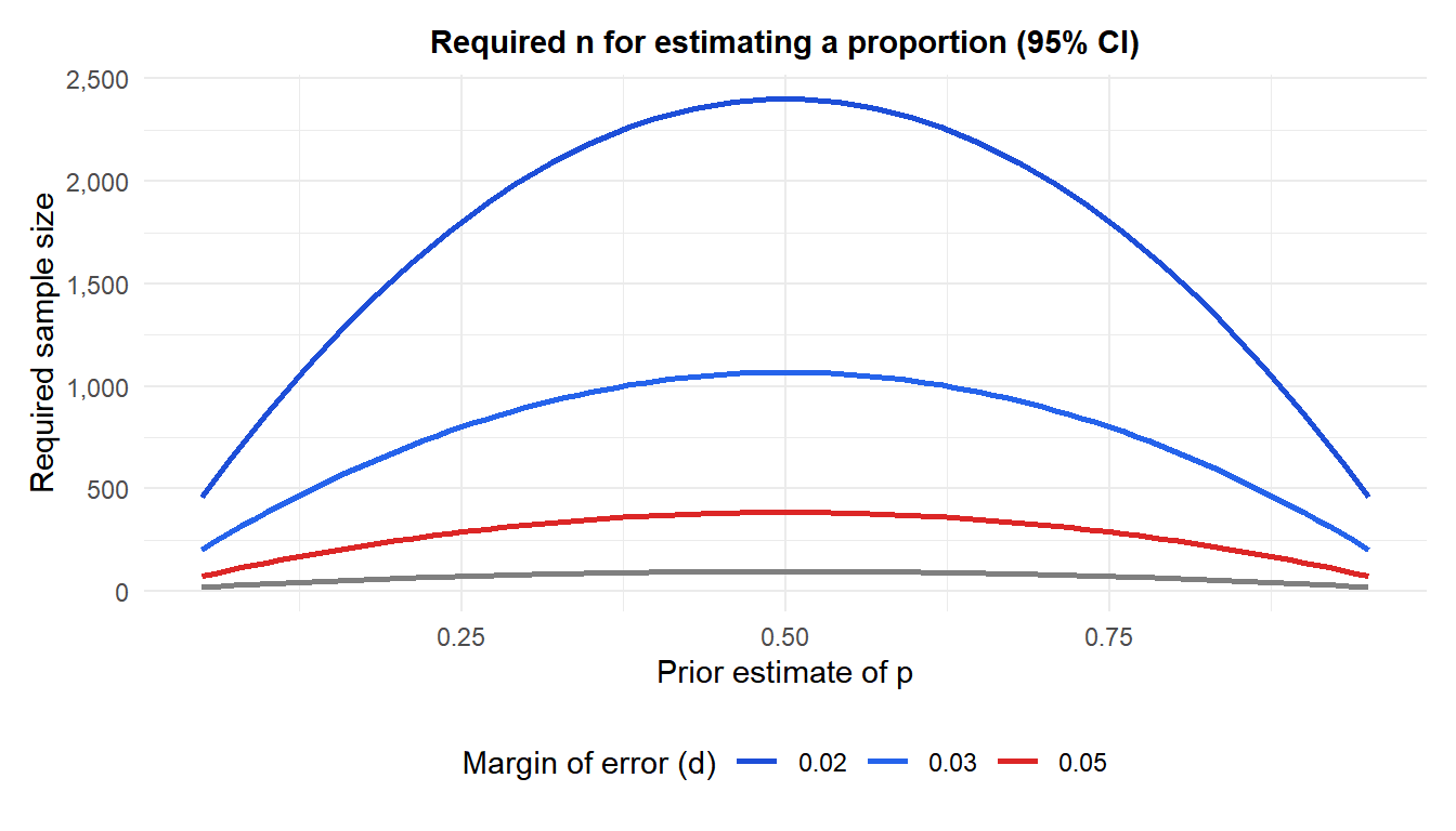
The chart shows that the maximum required \(n\) always occurs at \(p = 0.5\), and that decreasing \(d\) from 5% to 2% roughly quadruples the required sample size.
A factory wants to estimate its defect rate to within \(\pm 2\%\) at 95% confidence. A previous audit found a defect rate of about 8%.
Using the prior estimate \(p = 0.08\):
\[n \geq \frac{1.960^2 \times 0.08 \times 0.92}{0.02^2} = \frac{3.842 \times 0.0736}{0.0004} = \frac{0.2828}{0.0004} \approx 707\]
Using the conservative \(p = 0.5\):
\[n \geq \frac{1.960^2 \times 0.25}{0.02^2} = \frac{0.9604}{0.0004} = 2{,}401\]
The prior estimate saves 1,694 inspections. When \(p\) is far from 0.5, using prior information is efficient.
Sample size for comparing two means
To detect a difference of \(\delta = \mu_1 - \mu_2\) with margin of error \(d\) at confidence \(1-\alpha\), assuming equal sample sizes \(n_1 = n_2 = n\) and equal variances \(\sigma^2\):
\[n \geq 2\left(\frac{z_{\alpha/2} \cdot \sigma}{d}\right)^2\]
For a hypothesis test that detects a difference \(\delta\) with power \(1-\beta\):
\[n \geq \frac{2\sigma^2(z_{\alpha/2} + z_\beta)^2}{\delta^2}\]
where \(z_\beta\) is the standard normal quantile for the desired power (e.g. \(z_{0.80} = 0.842\) for 80% power, \(z_{0.90} = 1.282\) for 90% power).
A trial compares blood pressure reduction between two drugs. From prior data, \(\sigma \approx 12\) mmHg. The clinically meaningful difference is \(\delta = 5\) mmHg. Design the trial with 95% confidence and 80% power.
\[n \geq \frac{2 \times 144 \times (1.960 + 0.842)^2}{25} = \frac{288 \times 7.852}{25} = \frac{2{,}261}{25} \approx 91\]
Each group needs at least 91 patients (182 total). For 90% power:
\[n \geq \frac{2 \times 144 \times (1.960 + 1.282)^2}{25} = \frac{288 \times 10.511}{25} \approx 121 \text{ per group}\]
Going from 80% to 90% power increases the total sample from 182 to 242.
Practical considerations
⚠️ The calculated n is a minimum, not a target
The formula gives the minimum \(n\) under ideal conditions. In practice, always inflate it to account for:
- Dropout and non-response: if you expect 15% dropout, divide by 0.85. A study needing 148 complete observations requires enrolling \(148/0.85 \approx 175\) participants.
- Multiple comparisons: if you test several hypotheses, the effective \(\alpha\) per test is lower, requiring larger \(n\).
- Cluster sampling: observations within clusters are correlated. Multiply \(n\) by the design effect \(\text{DEFF} = 1 + (m-1)\rho\), where \(m\) is the cluster size and \(\rho\) is the intraclass correlation.
- Subgroup analyses: if you need to estimate parameters within subgroups, each subgroup needs its own minimum \(n\).
A good rule of thumb: calculate the minimum \(n\), add 20% as a buffer, then review feasibility.
💡 What to do when the required n is too large
If the calculated sample size exceeds your budget or timeline:
- Increase \(d\): accept a wider margin of error. Doubling \(d\) quarters \(n\).
- Reduce the confidence level: going from 99% to 95% reduces \(n\) by about 30%.
- Use a better prior for \(p\) or \(\sigma\): a pilot study to estimate variability can substantially reduce the required \(n\).
- Use a one-sided test: if only one direction matters, \(z_{\alpha}\) instead of \(z_{\alpha/2}\) reduces \(n\).
- Accept lower power: reducing power from 90% to 80% saves roughly 25% of observations in a two-sample test.
Document any compromises explicitly: reviewers and regulators will ask.

