What is an estimator?
An estimator is a function of the sample data used to approximate an unknown population parameter. Choosing a good estimator is not obvious: two different estimators of the same parameter can have very different accuracy, variance, and behavior under assumptions violations.
Definition
A population parameter is a fixed, unknown characteristic of a population: the mean \(\mu\), the variance \(\sigma^2\), the proportion \(p\), and so on. Since we cannot measure the entire population, we collect a sample \(x_1, x_2, \ldots, x_n\) and use a function of those observations to approximate the parameter.
An estimator \(\hat{\theta}\) is any function of the sample data used to estimate a population parameter \(\theta\):
\[\hat{\theta} = g(x_1, x_2, \ldots, x_n)\]
The result of applying the estimator to a specific dataset is called an estimate. The estimator is the rule; the estimate is the number.
⚠️ Estimator vs estimate: two different things
An estimator is a random variable: before collecting data, it can take many possible values depending on which sample you happen to draw. An estimate is the specific value the estimator takes once you have your data.
The sample mean \(\bar{X} = \frac{1}{n}\sum X_i\) is an estimator. The value \(\bar{x} = 47.3\) computed from a specific dataset is an estimate. This distinction matters when discussing properties like unbiasedness, which is a property of the estimator (its average behavior across all possible samples), not of any single estimate.
Estimators fall into two broad categories:
- Point estimators: produce a single value as the estimate (\(\hat{\mu} = \bar{x}\)).
- Interval estimators: produce a range of plausible values (confidence intervals).
This post focuses on point estimators.
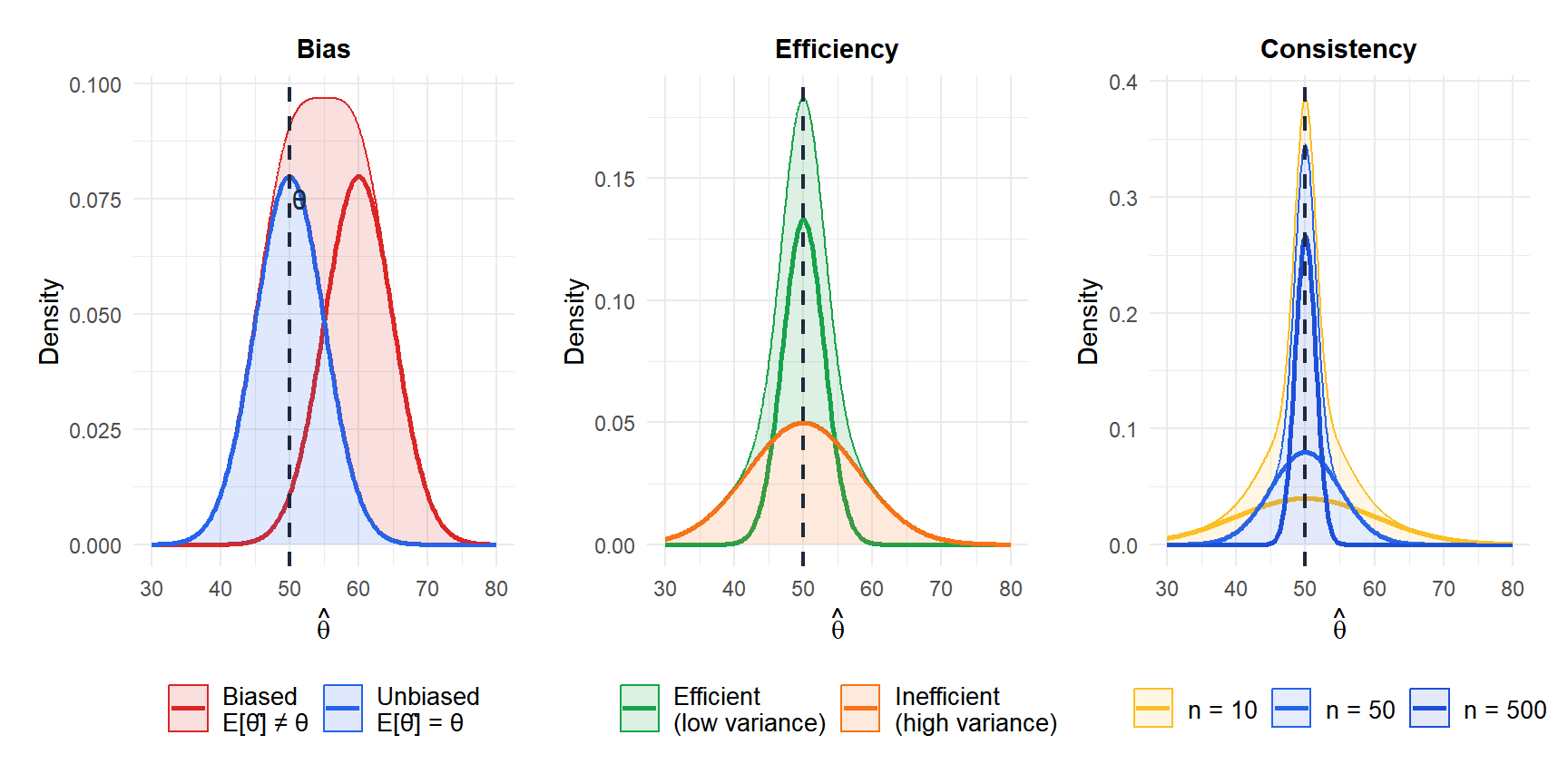
Desirable properties of estimators
- Unbiasedness
An estimator \(\hat{\theta}\) is unbiased if its expected value equals the true parameter:
\[E[\hat{\theta}] = \theta\]
The sample mean \(\bar{X}\) is an unbiased estimator of \(\mu\): on average across all possible samples, it hits the target. The sample variance \(S^2 = \frac{1}{n-1}\sum(X_i - \bar{X})^2\) is an unbiased estimator of \(\sigma^2\): note the \(n-1\) in the denominator (Bessel’s correction). Using \(n\) instead gives a biased estimator.
- Consistency
An estimator is consistent if it converges to the true value as the sample size grows:
\[\lim_{n \to \infty} P(|\hat{\theta} - \theta| > \varepsilon) = 0 \quad \text{for any } \varepsilon > 0\]
A consistent estimator gets more accurate with more data. The sample mean is consistent for \(\mu\); the sample median is also consistent for \(\mu\) in symmetric distributions.
- Efficiency
Among all unbiased estimators, the efficient estimator has the smallest variance. The theoretical lower bound is given by the Cramér-Rao bound:
\[\text{Var}(\hat{\theta}) \geq \frac{1}{I(\theta)}\]
where \(I(\theta)\) is the Fisher information. An estimator that achieves this bound is called minimum variance unbiased estimator (MVUE). For normally distributed data, \(\bar{X}\) is the MVUE for \(\mu\).
- Sufficiency
An estimator is sufficient if it captures all the information in the sample relevant to \(\theta\). Once you know a sufficient statistic, the rest of the data adds nothing. The sample mean is sufficient for \(\mu\) in normal populations.
- Robustness
A robust estimator performs well even when assumptions are violated, particularly in the presence of outliers. The median is more robust than the mean: a single extreme observation can pull the mean far from the center but barely moves the median.
Mean squared error
In practice, unbiasedness and efficiency are often in tension: a slightly biased estimator with much lower variance can be more useful than an unbiased estimator with high variance. The mean squared error (MSE) unifies both:
\[\text{MSE}(\hat{\theta}) = E[(\hat{\theta} - \theta)^2] = \text{Var}(\hat{\theta}) + \text{Bias}(\hat{\theta})^2\]
A good estimator minimizes MSE, not necessarily bias alone. This is the foundation of the bias-variance tradeoff, central to both classical statistics and machine learning.
Two estimators for the population variance \(\sigma^2\):
- \(S^2 = \frac{1}{n-1}\sum(X_i - \bar{X})^2\): unbiased, \(E[S^2] = \sigma^2\).
- \(\hat{\sigma}^2 = \frac{1}{n}\sum(X_i - \bar{X})^2\): biased, \(E[\hat{\sigma}^2] = \frac{n-1}{n}\sigma^2\).
The biased estimator has slightly smaller variance. For large \(n\) the difference is negligible, but for small samples the unbiased version is preferred. In maximum likelihood estimation, \(\hat{\sigma}^2\) (with \(n\) in the denominator) is typically used, accepting a small bias in exchange for other favorable properties.
Common estimators
| Parameter | Estimator | Unbiased? | Notes |
|---|---|---|---|
| Mean \(\mu\) | \(\bar{X} = \frac{1}{n}\sum X_i\) | Yes | MVUE for normal data |
| Variance \(\sigma^2\) | \(S^2 = \frac{1}{n-1}\sum(X_i-\bar{X})^2\) | Yes | Bessel’s correction |
| Proportion \(p\) | \(\hat{p} = X/n\) | Yes | \(X\) = number of successes |
| Median | Sample median | Yes (symmetric dist.) | More robust than mean |
| Max of Uniform\((0,\theta)\) | \(\frac{n+1}{n}X_{(n)}\) | Yes | MLE \(X_{(n)}\) is biased |
💡 How to choose between estimators
No single criterion dominates in all situations:
- If assumptions hold (normality, no outliers): prefer the MVUE, usually the sample mean.
- If data has heavy tails or outliers: prefer robust estimators (median, trimmed mean).
- If sample size is small: unbiasedness matters more; prefer \(S^2\) over \(\hat{\sigma}^2\).
- If prediction accuracy matters more than interpretability: minimize MSE, accepting some bias.
In practice, it helps to examine the data, check assumptions, and compare estimators using simulation when the best choice is not clear.

