Confidence interval for variances ratio
The confidence interval for \(\sigma_1^2/\sigma_2^2\) uses the F distribution and is always asymmetric: the upper bound is further from the observed ratio than the lower bound. It is used to compare the variability of two independent processes and to check the equal-variance assumption before a pooled \(t\)-test.
Formula
Given two independent samples with sample variances \(S_1^2\) (\(n_1\) observations) and \(S_2^2\) (\(n_2\) observations), the statistic:
\[F = \frac{S_1^2/\sigma_1^2}{S_2^2/\sigma_2^2} \sim F(n_1-1,\; n_2-1)\]
Inverting this pivot gives a \((1-\alpha)\) CI for \(\sigma_1^2/\sigma_2^2\):
\[\left(\frac{S_1^2}{S_2^2} \cdot \frac{1}{F_{1-\alpha/2,\; n_1-1,\; n_2-1}},\;\; \frac{S_1^2}{S_2^2} \cdot \frac{1}{F_{\alpha/2,\; n_1-1,\; n_2-1}}\right)\]
Note the order: the larger F critical value (\(F_{1-\alpha/2}\)) divides into the lower bound, and the smaller (\(F_{\alpha/2}\)) divides into the upper bound.
The reciprocal relationship of the F distribution gives: \(F_{\alpha/2,\; d_1,\; d_2} = 1/F_{1-\alpha/2,\; d_2,\; d_1}\), which is useful when only upper-tail F tables are available.
⚠️ The F test for variances is extremely sensitive to non-normality
Unlike the \(t\)-test for means (which is fairly robust to non-normality thanks to the CLT), the F test for variances is not robust at all. Non-normal data can produce highly significant F statistics even when the population variances are equal, and vice versa.
If normality is in doubt:
- Use Levene’s test (based on absolute deviations from the median): robust to non-normality, available in R as
leveneTest()from thecarpackage. - Use Bartlett’s test for normal data, Levene’s or Fligner-Killeen for non-normal data.
- For the CI itself, consider a bootstrap confidence interval for the ratio.
F distribution and the CI
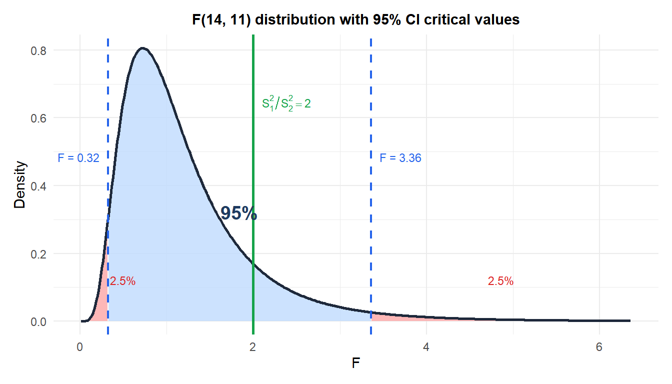
The F distribution is right-skewed and always positive. The 95% CI for the variance ratio is defined by the two critical values that leave 2.5% in each tail. The observed ratio \(S_1^2/S_2^2\) (green line) falls inside the central region in this example, confirming that 1 is within the CI.
Step-by-step example
A quality engineer compares the consistency of two production lines. Line 1 (\(n_1 = 15\)) has \(S_1^2 = 4.0\) mm² and Line 2 (\(n_2 = 12\)) has \(S_2^2 = 2.0\) mm². Construct a 95% CI for \(\sigma_1^2/\sigma_2^2\).
Step 1: compute the observed ratio.
\[F_{\text{obs}} = \frac{S_1^2}{S_2^2} = \frac{4.0}{2.0} = 2.0\]
Step 2: find the F critical values with \(df_1 = 14\), \(df_2 = 11\).
\[F_{0.975,\; 14,\; 11} = 3.095, \qquad F_{0.025,\; 14,\; 11} = 0.305\]
In R: qf(0.975, 14, 11) and qf(0.025, 14, 11).
Step 3: compute the bounds.
\[\text{Lower} = \frac{2.0}{3.095} \approx 0.646, \qquad \text{Upper} = \frac{2.0}{0.305} \approx 6.557\]
\[\text{95\% CI for } \sigma_1^2/\sigma_2^2: (0.65,\; 6.56)\]
Since the CI includes 1, there is no significant evidence that the two lines differ in variability at the 5% level. However, the wide interval reflects limited sample sizes: Line 1 could have anywhere from 65% to 656% the variance of Line 2.
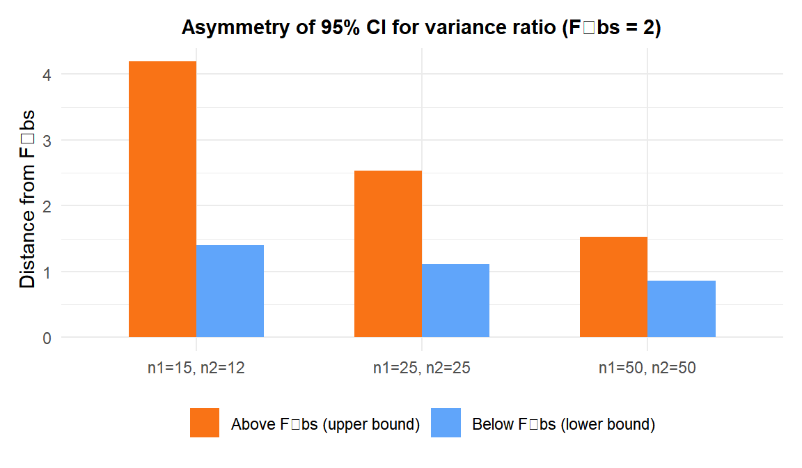
The upper bound extends further from \(F_\text{obs}\) than the lower bound in all cases: the asymmetry of the F distribution makes this CI always asymmetric, and it is more pronounced for smaller samples.
A pharmaceutical company compares the batch-to-batch variability of two manufacturing processes. Process A (\(n_1 = 30\), \(S_1^2 = 12.4\)) vs Process B (\(n_2 = 30\), \(S_2^2 = 4.1\)).
\[F_\text{obs} = 12.4/4.1 \approx 3.02\]
\[F_{0.975,\; 29,\; 29} \approx 2.101, \quad F_{0.025,\; 29,\; 29} \approx 0.476\]
\[\text{CI} = \left(\frac{3.02}{2.101},\; \frac{3.02}{0.476}\right) = (1.44,\; 6.34)\]
The CI excludes 1: Process A is significantly more variable than Process B. The ratio is between 1.44 and 6.34, meaning Process A has between 44% and 534% more variance than Process B.
💡 Practical guidelines
- The CI for a variance ratio is most useful for checking the equal-variance assumption before a pooled \(t\)-test. If 1 is inside the CI, the pooled test is defensible; if 1 is outside, use Welch.
- For comparing variances as a primary objective (not just as an assumption check), Levene’s test is preferred due to its robustness to non-normality.
- In R:
var.test(x, y)computes both the F statistic and its CI.car::leveneTest(y ~ group)provides the robust alternative. - The CI is only valid when both populations are normal. For non-normal data, bootstrap the ratio \(S_1^2/S_2^2\) directly.

