Confidence interval for the difference between two means
The confidence interval for \(\mu_1 - \mu_2\) estimates the range of plausible values for the true difference between two population means. Whether to use a pooled or Welch approach depends on whether the population variances can be assumed equal.
Setup
We have two independent random samples:
- Group 1: \(n_1\) observations, sample mean \(\bar{X}_1\), sample variance \(S_1^2\).
- Group 2: \(n_2\) observations, sample mean \(\bar{X}_2\), sample variance \(S_2^2\).
The point estimate of \(\mu_1 - \mu_2\) is \(\bar{X}_1 - \bar{X}_2\). The CI takes the form:
\[(\bar{X}_1 - \bar{X}_2) \pm t^* \cdot \text{SE}(\bar{X}_1 - \bar{X}_2)\]
The two approaches differ in how they compute \(\text{SE}\) and the degrees of freedom for \(t^*\).
Welch’s interval (unequal variances)
When the population variances may differ, use Welch’s \(t\)-interval:
\[\text{SE} = \sqrt{\frac{S_1^2}{n_1} + \frac{S_2^2}{n_2}}\]
The degrees of freedom are given by the Satterthwaite approximation:
\[df = \frac{\left(\frac{S_1^2}{n_1} + \frac{S_2^2}{n_2}\right)^2}{\frac{(S_1^2/n_1)^2}{n_1-1} + \frac{(S_2^2/n_2)^2}{n_2-1}}\]
This is always a non-integer and must be rounded down. Welch’s interval is the default in R (t.test()) and most statistical software.
Pooled interval (equal variances)
When the population variances can be assumed equal (\(\sigma_1^2 = \sigma_2^2 = \sigma^2\)), pool the two sample variances into one estimate:
\[S_p^2 = \frac{(n_1-1)S_1^2 + (n_2-1)S_2^2}{n_1+n_2-2}\]
\[\text{SE} = S_p\sqrt{\frac{1}{n_1} + \frac{1}{n_2}}, \qquad df = n_1 + n_2 - 2\]
The pooled interval is slightly narrower than Welch when variances are truly equal, but can be misleading when they differ.
⚠️ Default to Welch: the equal variance assumption is rarely justified
Using the pooled interval when variances are unequal gives incorrect coverage: the actual CI may be narrower than stated and miss the true difference more often than the nominal \(\alpha\) level implies.
The rule “use pooled when \(n < 30\), use Welch when \(n \geq 30\)” is outdated and incorrect. The right rule: always use Welch unless there is a strong prior reason to assume equal variances (same instrument, same process, randomized experiment with equal allocation). In R, t.test(..., var.equal = FALSE) is the default and the correct choice in most situations.
Visualizing the two groups
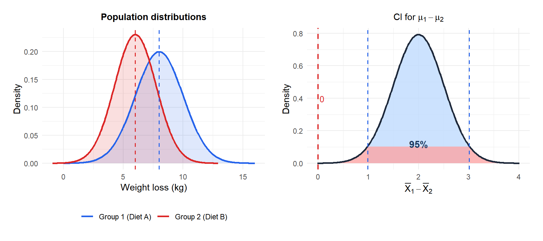
The right panel shows the sampling distribution of the difference \(\bar{X}_1 - \bar{X}_2\). The red dashed line at 0 represents “no difference”. Since 0 falls outside the 95% CI, the difference is statistically significant at the 5% level.
Step-by-step example
A clinical trial compares two diets over 6 months:
- Diet A: \(n_1 = 30\), \(\bar{x}_1 = 8.0\) kg, \(S_1 = 2.0\) kg.
- Diet B: \(n_2 = 25\), \(\bar{x}_2 = 6.0\) kg, \(S_2 = 1.73\) kg.
Construct a 95% CI for \(\mu_A - \mu_B\).
Step 1: compute the point estimate.
\[\bar{x}_1 - \bar{x}_2 = 8.0 - 6.0 = 2.0 \text{ kg}\]
Step 2: compute the Welch SE.
\[\text{SE} = \sqrt{\frac{4.0}{30} + \frac{3.0}{25}} = \sqrt{0.1333 + 0.1200} = \sqrt{0.2533} \approx 0.503 \text{ kg}\]
Step 3: Satterthwaite degrees of freedom.
\[df = \frac{0.2533^2}{\frac{(0.1333)^2}{29} + \frac{(0.1200)^2}{24}} = \frac{0.0641}{\frac{0.01777}{29} + \frac{0.0144}{24}} \approx \frac{0.0641}{0.000613 + 0.000600} \approx 52.8 \to 52\]
Step 4: critical value.
\[t_{0.025,\; 52} \approx 2.007\]
Step 5: construct the CI.
\[\text{CI} = 2.0 \pm 2.007 \times 0.503 = 2.0 \pm 1.01 = (0.99,\; 3.01) \text{ kg}\]
The CI does not include 0, so there is a statistically significant difference. Diet A produces between 0.99 and 3.01 kg more weight loss than Diet B, on average, with 95% confidence.
Same data as above but now assuming equal variances for the pooled approach:
\[S_p^2 = \frac{29 \times 4.0 + 24 \times 3.0}{53} = \frac{116 + 72}{53} = \frac{188}{53} \approx 3.547\]
\[\text{SE}_p = \sqrt{3.547 \times (1/30 + 1/25)} = \sqrt{3.547 \times 0.0733} \approx 0.510 \text{ kg}\]
\[df_p = 53, \quad t_{0.025,\; 53} \approx 2.006\]
\[\text{CI}_{\text{pooled}} = 2.0 \pm 2.006 \times 0.510 = (0.978,\; 3.022)\]
In this case the two intervals are nearly identical because \(S_1^2 \approx S_2^2\). When variances differ substantially, the gap between Welch and pooled intervals can be large.
💡 Interpreting the CI for a difference
Three cases tell the whole story:
- CI entirely above 0: \(\mu_1 > \mu_2\) is supported (Group 1 has a higher mean).
- CI entirely below 0: \(\mu_1 < \mu_2\) is supported (Group 2 has a higher mean).
- CI includes 0: the data are consistent with no difference at this confidence level.
A CI that just barely excludes 0 is very different from one that excludes it by a wide margin. Always report the actual interval, not just whether it includes 0.

