Poisson distribution
The Poisson distribution models the number of events occurring in a fixed interval of time or space, when events happen independently and at a constant average rate. It is widely used in queuing theory, reliability engineering, epidemiology, and telecommunications.
Definition
A random variable \(X\) follows a Poisson distribution with parameter \(\lambda > 0\), written \(X \sim \text{Poisson}(\lambda)\), if:
\[P(X = k) = \frac{\lambda^k e^{-\lambda}}{k!}, \quad k = 0, 1, 2, \ldots\]
where \(\lambda\) is the expected number of events in the interval, \(k\) is the observed count, and \(e \approx 2.71828\) is Euler’s number.
The Poisson distribution requires three conditions:
- Events occur independently: one event does not make another more or less likely.
- The average rate \(\lambda\) is constant throughout the interval.
- Two events cannot occur at exactly the same instant (no simultaneous events).
Probability Mass Function and CDF
The PMF gives the probability of exactly \(k\) events. The CDF accumulates these:
\[F(k) = P(X \leq k) = \sum_{i=0}^{k} \frac{\lambda^i e^{-\lambda}}{i!}\]
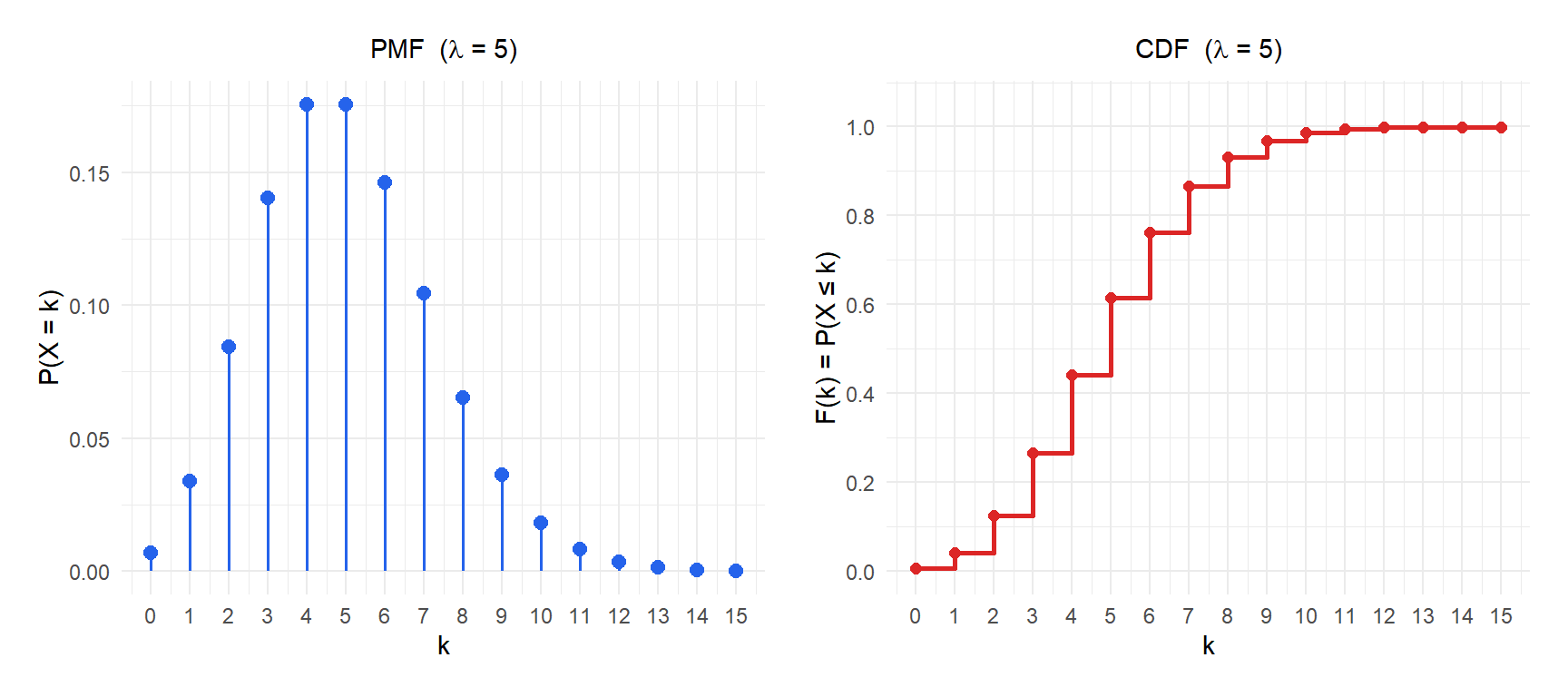
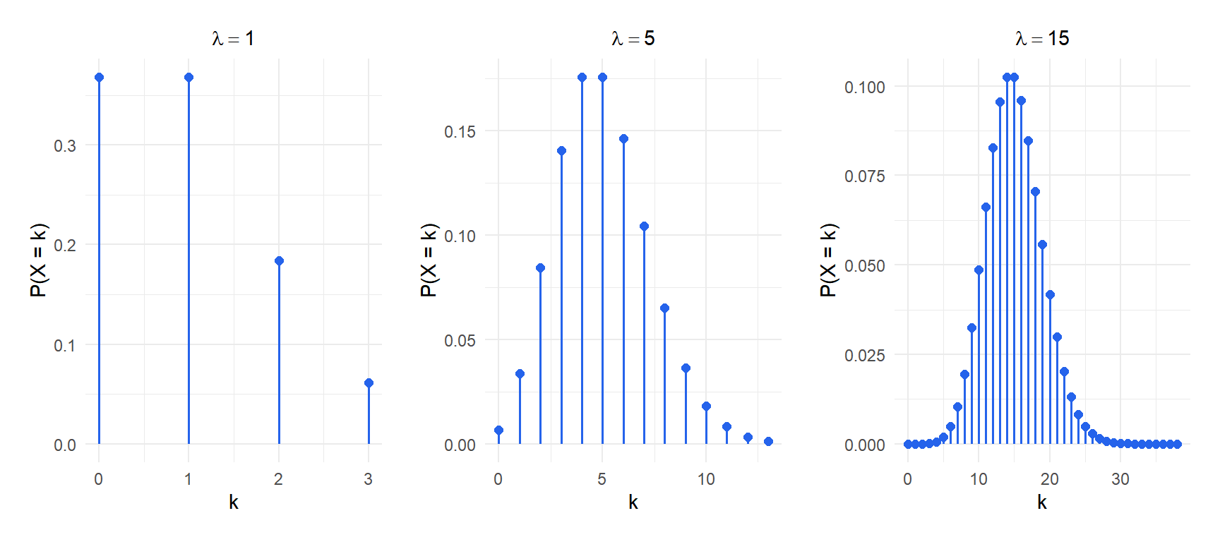
Figure 1: As lambda increases, the Poisson distribution shifts right and becomes more symmetric
Properties
For \(X \sim \text{Poisson}(\lambda)\):
- Expected Value (Mean)
\[E(X) = \lambda\]
- Variance
\[\text{Var}(X) = \lambda\]
The mean and variance are equal. This is the defining characteristic of the Poisson distribution and the basis for checking whether data is Poisson-distributed.
- Skewness
\[\text{Skewness} = \frac{1}{\sqrt{\lambda}}\]
The distribution is right-skewed for small \(\lambda\) and becomes increasingly symmetric as \(\lambda\) grows.
- Kurtosis
\[g_2 = \frac{1}{\lambda}\]
- Mode
\(\lfloor \lambda \rfloor\) if \(\lambda\) is not an integer. If \(\lambda\) is an integer, both \(\lambda\) and \(\lambda - 1\) are modes.
- Quantile Function
No closed-form expression exists. Computed numerically by most software.
Step-by-step example
A hospital emergency department receives an average of 8 patients per hour during night shifts. Let \(X \sim \text{Poisson}(8)\).
Probability of exactly 5 arrivals in one hour:
\[P(X = 5) = \frac{8^5 e^{-8}}{5!} = \frac{32768 \times 0.000335}{120} \approx 0.0916\]
About 9.2% chance of exactly 5 arrivals.
Probability of 10 or more arrivals (overloaded shift):
\[P(X \geq 10) = 1 - P(X \leq 9) = 1 - F(9) \approx 1 - 0.717 = 0.283\]
Nearly 28% of night shifts will have 10 or more arrivals.
Expected arrivals and standard deviation:
\[E(X) = 8, \qquad \text{SD}(X) = \sqrt{8} \approx 2.83\]
- Call center: a support line receives 12 calls per hour on average. \(X \sim \text{Poisson}(12)\). Probability of exactly 10 calls: \(P(X=10) \approx 0.105\).
- Website errors: a server logs an average of 2 errors per day. \(X \sim \text{Poisson}(2)\). Probability of zero errors: \(P(X=0) = e^{-2} \approx 0.135\).
- Radioactive decay: a Geiger counter registers an average of 3 particles per second. \(X \sim \text{Poisson}(3)\). Probability of 5 or more: \(P(X \geq 5) \approx 0.185\).
Assumptions and limitations
⚠️ Overdispersion: when Var(X) > E(X)
The Poisson distribution assumes \(\text{Var}(X) = E(X)\). In practice, count data often shows overdispersion: the variance is larger than the mean. This happens when events are not truly independent (disease cases cluster in households, accidents cluster at specific locations) or when \(\lambda\) varies across observations.
If you fit a Poisson model and find overdispersion, use the negative binomial distribution instead. Ignoring overdispersion leads to standard errors that are too small and p-values that are too optimistic.
⚠️ The rate must be constant over the interval
The Poisson distribution assumes (\lambda) is constant. If the rate changes over time (more calls in the morning than at night, more accidents in rain), a single Poisson model is not appropriate. Consider splitting the interval, using a non-homogeneous Poisson process, or including covariates in a Poisson regression model.
Poisson as an approximation to the Binomial
When \(n\) is large and \(p\) is small, the binomial distribution is well approximated by a Poisson with \(\lambda = np\):
\[\text{Binomial}(n, p) \approx \text{Poisson}(np) \quad \text{when } n \text{ large, } p \text{ small}\]
A common rule of thumb: \(n \geq 20\) and \(p \leq 0.05\).
A factory produces 10,000 components per day. Each has a 0.03% probability of being defective independently. The exact model is (X \sim \text{Binomial}(10000, 0.0003)), but the Poisson approximation (X \sim \text{Poisson}(3)) gives virtually identical probabilities and is much simpler to work with.
\(P(X = 0) = e^{-3} \approx 0.050\) (Poisson) vs \(0.0497\) (exact Binomial). The approximation error is negligible.
💡 Relationship with other distributions
- Binomial: Poisson is the limit of Binomial\((n, p)\) as \(n \to \infty\) and \(p \to 0\) with \(np = \lambda\) fixed.
- Normal approximation: for large \(\lambda\), \(\text{Poisson}(\lambda) \approx \mathcal{N}(\lambda, \lambda)\).
- Negative binomial: use when data shows overdispersion (\(\text{Var}(X) > E(X)\)).
- Exponential: if events follow a Poisson process with rate \(\lambda\), the time between consecutive events follows an Exponential\((\lambda)\) distribution.

