Geometric distribution
The geometric distribution models the waiting time until the first success in a sequence of independent Bernoulli trials. It is the only discrete distribution with the memoryless property: past failures carry no information about future outcomes.
Definition
There are two common versions of the geometric distribution. Both describe the same process but count different things:
Version 1: number of trials until the first success (\(X \geq 1\)):
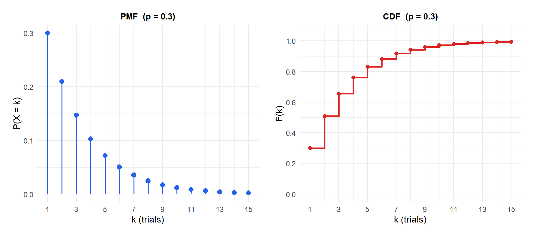
\[P(X = k) = (1-p)^{k-1} p, \quad k = 1, 2, 3, \ldots\]
Version 2: number of failures before the first success (\(X \geq 0\)):
\[P(X = k) = (1-p)^{k} p, \quad k = 0, 1, 2, \ldots\]
Both are called “geometric distribution.” Version 2 is a special case of the negative binomial with \(r = 1\).
⚠️ Which parametrization does your software use?
R’s dgeom(x, prob = p) uses version 2: \(x\) is the number of failures before the first success. So dgeom(0, p) gives \(P(X=0) = p\), the probability of success on the very first trial.
If you want version 1 (number of trials), use dgeom(x - 1, prob = p) or equivalently note that if \(Y\) is version 2, then \(X = Y + 1\) is version 1.
This off-by-one difference is a frequent source of errors in exam calculations and in code.
Probability Mass Function and CDF
Using version 1 (\(k\) = number of trials), the CDF has a clean closed form:
\[F(k) = P(X \leq k) = 1 - (1-p)^k\]
This means the probability of needing more than \(k\) trials is simply \((1-p)^k\).
Properties
For \(X \sim \text{Geometric}(p)\) using version 1 (number of trials):
- Expected Value (Mean)
\[E(X) = \frac{1}{p}\]
If success probability is 20%, you need on average 5 trials to get the first success.
- Variance
\[\text{Var}(X) = \frac{1-p}{p^2}\]
- Skewness
\[\text{Skewness} = \frac{2-p}{\sqrt{1-p}}\]
Always positive: the distribution has a long right tail regardless of \(p\).
- Kurtosis
\[g_2 = 6 + \frac{p^2}{1-p}\]
- CDF (closed form)
\[F(k) = 1 - (1-p)^k\]
- Quantile Function
\[Q(u) = \left\lceil \frac{\log(1-u)}{\log(1-p)} \right\rceil\]
where \(\lceil \cdot \rceil\) is the ceiling function.
The memoryless property
The geometric distribution is the only discrete distribution with the memoryless property:
\[P(X > m + n \mid X > m) = P(X > n)\]
This means: if you have already failed \(m\) times, the probability of needing more than \(n\) additional trials is exactly the same as if you were starting fresh. Past failures provide zero information about future outcomes.
A quality inspector tests components one by one. Each has a 10% defect rate. The inspector has already tested 20 components without finding a defect.
What is the probability of needing more than 5 additional tests?
By the memoryless property: \(P(X > 5) = (1 - 0.1)^5 = 0.9^5 \approx 0.590\).
The 20 previous tests are completely irrelevant. The geometric distribution has no memory of past failures.
⚠️ The memoryless property can be counterintuitive
Many students expect that after many failures, a success becomes “due.” This intuition is wrong for geometric processes. A fair coin has no memory: after 10 tails in a row, the probability of heads on the next flip is still 0.5. The gambler’s fallacy is exactly the belief that geometric (memoryless) processes do have memory.
Step-by-step example
A data center experiences server failures that require a reboot. Each reboot attempt succeeds with probability \(p = 0.4\). Let \(X\) = number of attempts until the first successful reboot, \(X \sim \text{Geometric}(0.4)\).
Probability of success on exactly the 3rd attempt:
\[P(X = 3) = (1-0.4)^{3-1} \times 0.4 = 0.6^2 \times 0.4 = 0.36 \times 0.4 = 0.144\]
Expected number of attempts:
\[E(X) = \frac{1}{0.4} = 2.5 \text{ attempts}\]
Probability of needing more than 4 attempts:
\[P(X > 4) = (1-0.4)^4 = 0.6^4 = 0.1296\]
About 13% of failures will require more than 4 reboot attempts.
Probability of success within the first 3 attempts:
\[F(3) = 1 - (1-0.4)^3 = 1 - 0.216 = 0.784\]
Nearly 78% of failures are resolved within 3 attempts.
- A/B testing: a new ad variant has a 5% click-through rate. Expected number of impressions before the first click: \(E(X) = 1/0.05 = 20\).
- Job interviews: a candidate passes each interview stage with probability 0.3. Probability of passing on the first try: \(P(X=1) = 0.3\). Expected number of attempts: \(1/0.3 \approx 3.3\).
- Network retransmission: a data packet is successfully delivered with probability 0.95 per attempt. Probability of needing more than 2 attempts: \((1-0.95)^2 = 0.0025\).
💡 Relationship with other distributions
- Negative Binomial: Geometric\((p)\) = NegBin\((1, p)\). The geometric is the special case with \(r = 1\).
- Exponential: the continuous analogue of the geometric distribution. Both are memoryless: geometric for discrete trials, exponential for continuous time.
- Binomial: if you run \(n\) geometric trials and count successes, you get a binomial. The geometric asks “when is the first success?”; the binomial asks “how many successes in \(n\) trials?”.

