Discrete uniform distribution
The discrete uniform distribution assigns equal probability to each outcome in a finite set. It is the simplest discrete distribution and the mathematical foundation of any process where all outcomes are equally likely.
Definition
A random variable \(X\) follows a discrete uniform distribution over a set of \(n\) values \(\{x_1, x_2, \ldots, x_n\}\) if every value has the same probability:
\[P(X = x_i) = \frac{1}{n}, \quad i = 1, 2, \ldots, n\]
The most common parametrization uses integer values from \(a\) to \(b\), giving \(n = b - a + 1\) equally likely outcomes. This is written \(X \sim \text{Uniform}(a, b)\).
Probability Mass Function and CDF
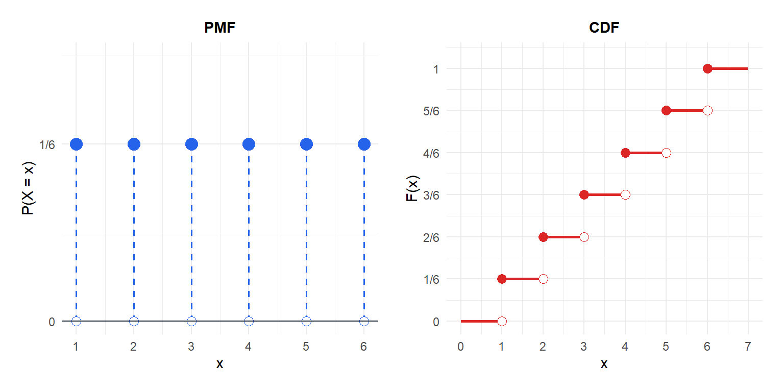
The PMF is constant across all possible values:
\[P(X = x) = \frac{1}{n} \quad \text{for } x \in \{a, a+1, \ldots, b\}\]
The cumulative distribution function gives the probability of being at or below a given value:
\[F(x) = \frac{\lfloor x \rfloor - a + 1}{n} \quad \text{for } a \leq x \leq b\]
where \(\lfloor x \rfloor\) is the floor function. \(F(x) = 0\) for \(x < a\) and \(F(x) = 1\) for \(x > b\).
Properties
For \(X \sim \text{Uniform}(a, b)\) with \(n = b - a + 1\):
- Expected Value (Mean)
\[E(X) = \frac{a + b}{2}\]
- Variance
\[\text{Var}(X) = \frac{n^2 - 1}{12} = \frac{(b-a+1)^2 - 1}{12}\]
- Skewness
Always 0: the distribution is perfectly symmetric around its mean.
- Kurtosis
\[g_2 = -\frac{6(n^2+1)}{5(n^2-1)}\]
For large \(n\), kurtosis approaches \(-1.2\): the distribution is flatter than the normal (platykurtic).
- Quantile Function
\[Q(p) = a + \lfloor p \cdot n \rfloor\]
Example: rolling a fair die
A standard six-sided die gives \(X \sim \text{Uniform}(1, 6)\), with \(n = 6\).
- PMF: \(P(X = k) = 1/6 \approx 0.167\) for \(k = 1, 2, \ldots, 6\).
- Mean: \(E(X) = (1+6)/2 = 3.5\). In the long run, the average roll is 3.5.
- Variance: \(\text{Var}(X) = (36-1)/12 = 35/12 \approx 2.92\).
- CDF: \(F(4) = 4/6 \approx 0.667\). There is a 66.7% chance of rolling 4 or lower.
- Quantile: \(Q(0.5) = 1 + \lfloor 0.5 \times 6 \rfloor = 4\) (the median is 4).
- Random number generator: generating a random integer from 1 to 100 uniformly. Each integer has probability 1/100.
- Clinical trial randomization: assigning patients to treatment A or B randomly. Each patient has probability 1/2 of each assignment.
- Random sampling: drawing one employee ID from a list of 500. Each ID has probability 1/500.
- Lottery: choosing the winning number from 1 to 49 uniformly before any draws are made.
⚠️ Discrete uniform vs continuous uniform
Do not confuse these two distributions. The discrete uniform assigns probability (1/n) to each of (n) specific values. The continuous uniform assigns zero probability to any single point and only makes sense over intervals. A random integer from 1 to 6 is discrete uniform. The arrival time of a bus known only to be within a 10-minute window is continuous uniform. The formulas for mean, variance, and CDF are different in each case.
Sampling with and without replacement
Consecutive draws from a discrete uniform distribution are independent if sampling is done with replacement. If you roll a die twice, the second roll is completely unaffected by the first.
If sampling is without replacement (drawing cards from a deck without returning them), the outcomes are no longer uniform on the same set after each draw, and a hypergeometric model is more appropriate.
💡 When to use the discrete uniform distribution

