Chi-squared distribution
The chi-squared distribution arises naturally as the distribution of the sum of squared standard normal variables. It is the foundation of hypothesis tests for variance, goodness-of-fit tests, and tests of independence in contingency tables.
Definition
If \(Z_1, Z_2, \ldots, Z_\nu\) are independent standard normal random variables, then:
\[X = Z_1^2 + Z_2^2 + \cdots + Z_\nu^2 \sim \chi^2(\nu)\]
\(X\) follows a chi-squared distribution with \(\nu\) degrees of freedom. Its PDF is:
\[f(x) = \frac{x^{\nu/2 - 1} e^{-x/2}}{2^{\nu/2}\,\Gamma(\nu/2)}, \quad x > 0\]
The chi-squared distribution is a special case of the gamma distribution: \(\chi^2(\nu) = \text{Gamma}(\nu/2,\, 1/2)\).
The CDF has no closed form and is computed numerically. In practice, critical values are read from chi-squared tables or computed with software.
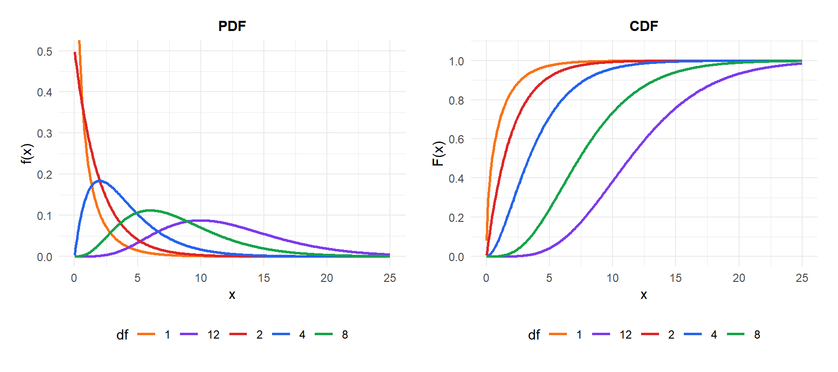
Effect of degrees of freedom
The degrees of freedom \(\nu\) fully determine the distribution:
- \(\nu = 1\) or \(\nu = 2\): strongly right-skewed, with the mode at 0 (\(\nu=1\)) or at \(x=0\) (\(\nu=2\), exponential case).
- Small \(\nu\): heavily right-skewed with a long right tail.
- Large \(\nu\): increasingly symmetric, approaching a normal distribution by the CLT.
Properties
For \(X \sim \chi^2(\nu)\):
- Expected Value (Mean)
\[E(X) = \nu\]
- Variance
\[\text{Var}(X) = 2\nu\]
- Skewness
\[\text{Skewness} = \sqrt{\frac{8}{\nu}}\]
Always positive. Decreases as \(\nu\) increases: the distribution becomes more symmetric for large \(\nu\).
- Kurtosis
\[g_2 = \frac{12}{\nu}\]
- Mode
\[\text{Mode} = \max(\nu - 2,\ 0)\]
For \(\nu \leq 2\), the mode is at 0.
- Quantile Function
No closed form; computed numerically. Common critical values are tabulated in chi-squared tables.
💡 Normal approximation for large ν
For large \(\nu\), the chi-squared distribution is well approximated by a normal:
\[\chi^2(\nu) \approx N(\nu, 2\nu)\]
A better approximation (Wilson-Hilferty) uses the cube root transformation:
\[\left(\frac{X}{\nu}\right)^{1/3} \approx N\!\left(1 - \frac{2}{9\nu},\ \frac{2}{9\nu}\right)\]
This approximation is accurate even for moderate \(\nu\) and is what most software uses internally.
Applications
Confidence interval and test for variance
If \(S^2\) is the sample variance of \(n\) observations from a \(N(\mu, \sigma)\) population, then:
\[\frac{(n-1)S^2}{\sigma^2} \sim \chi^2(n-1)\]
This leads to:
- A \((1-\alpha)\) confidence interval for \(\sigma^2\):
\[\left(\frac{(n-1)S^2}{\chi^2_{1-\alpha/2,\, n-1}},\ \frac{(n-1)S^2}{\chi^2_{\alpha/2,\, n-1}}\right)\]
- A hypothesis test \(H_0: \sigma^2 = \sigma_0^2\) using the test statistic \((n-1)S^2/\sigma_0^2\).
A lab measures 16 samples of a chemical compound. The sample standard deviation is \(S = 0.08\) mg/L. Construct a 95% CI for the population variance \(\sigma^2\).
With \(n = 16\) and \(\alpha = 0.05\):
- \(\chi^2_{0.975,\, 15} \approx 27.49\) and \(\chi^2_{0.025,\, 15} \approx 6.26\).
\[\text{CI} = \left(\frac{15 \times 0.0064}{27.49},\ \frac{15 \times 0.0064}{6.26}\right) = (0.0035,\ 0.0153)\]
The 95% CI for \(\sigma^2\) is \((0.0035, 0.0153)\) (mg/L)². For \(\sigma\): \((\sqrt{0.0035}, \sqrt{0.0153}) \approx (0.059, 0.124)\) mg/L.
Goodness-of-fit test
The Pearson chi-squared statistic:
\[\chi^2 = \sum_{i=1}^{k} \frac{(O_i - E_i)^2}{E_i}\]
follows a \(\chi^2(k-1)\) distribution under \(H_0\) (or \(\chi^2(k-1-p)\) if \(p\) parameters were estimated from the data). This is used to test whether observed frequencies match a hypothesized distribution.
Test of independence
For a contingency table with \(r\) rows and \(c\) columns, the same statistic follows \(\chi^2((r-1)(c-1))\) under independence. See the Pearson’s chi-squared test post for full details.
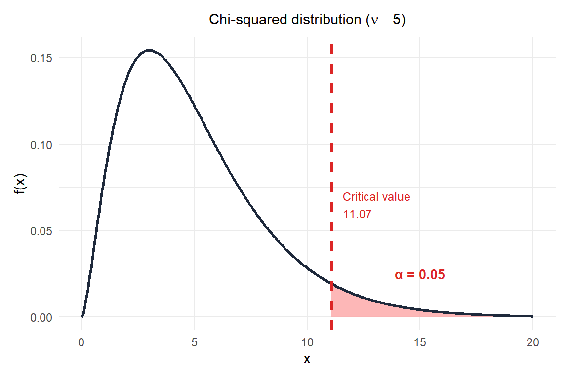
Figure 1: Chi-squared distribution with 5 degrees of freedom: rejection region at α=0.05 starts at the critical value 11.07
⚠️ Chi-squared tests require sufficient expected frequencies
All chi-squared tests assume that expected cell frequencies are large enough for the chi-squared approximation to be valid. The standard rule: all expected frequencies \(E_i \geq 5\). If this is violated, use exact tests (Fisher’s exact test for 2×2 tables, or exact multinomial tests for goodness-of-fit).
Step-by-step example: test for variance
A machine produces bolts with a specified diameter variance of \(\sigma_0^2 = 0.01\) mm². A quality engineer measures 25 bolts and finds \(S^2 = 0.015\) mm². Is there evidence that the variance has increased?
\(H_0: \sigma^2 = 0.01\) vs \(H_1: \sigma^2 > 0.01\) (one-sided test).
Test statistic:
\[\chi^2 = \frac{(n-1)S^2}{\sigma_0^2} = \frac{24 \times 0.015}{0.01} = 36\]
Critical value at \(\alpha = 0.05\) with \(\nu = 24\) df:
\[\chi^2_{0.95,\, 24} \approx 36.42\]
Since \(36 < 36.42\), we fail to reject \(H_0\) at the 5% level. The p-value is:
\[p = P(\chi^2_{24} > 36) \approx 0.053\]
Just above 5%. The evidence for increased variance is suggestive but not conclusive at this significance level.
💡 Relationship with other distributions
- Gamma: \(\chi^2(\nu) = \text{Gamma}(\nu/2, 1/2)\).
- Normal: sum of squared standard normals; for large \(\nu\), \(\chi^2(\nu) \approx N(\nu, 2\nu)\).
- Student’s t: if \(Z \sim N(0,1)\) and \(V \sim \chi^2(\nu)\) independently, then \(Z/\sqrt{V/\nu} \sim t(\nu)\).
- F distribution: ratio of two independent chi-squared variables divided by their degrees of freedom: \(F(\nu_1, \nu_2) = (\chi^2(\nu_1)/\nu_1) / (\chi^2(\nu_2)/\nu_2)\).
- Exponential: \(\chi^2(2) = \text{Exp}(1/2)\).

